Regime-conditional performance

Author: Artur Sepp

Implemented in qis — Quantitative Investment Strategies. Software citation: CITATION.cff.

Regime-conditional performance partitions the periods of a sample by what a benchmark did in each period and reports an asset’s performance within each part. In qis the default partition labels every quarter Bear, Normal or Bull by the full-sample 16% and 84% quantiles of the benchmark’s quarterly return, and the reported statistics are the regime frequencies, the conditional mean returns, and each regime’s contribution to the per-annum return and to the Sharpe ratio. Under the arithmetic and log conventions the Sharpe contributions add up exactly to the Sharpe ratio on the regime grid; under the default per-annum convention a residual is allocated so that the regime returns add up to the per-annum return.

Overview

A full-sample Sharpe ratio says how much return a strategy earned per unit of risk; it does not say when the return was earned. Two strategies with the same Sharpe ratio can earn it in opposite states of the world: one in the quarters in which equities fall, the other in quiet quarters, giving part of it back when equities fall. Sepp (2019) uses this distinction to separate the crisis beta of trend-following managers from the risk-premia alpha of alternative risk premia, and the regime decomposition of this chapter is the tool that makes the distinction measurable.

The calculation has three steps:

1. Classify. Resample the benchmark to a regime grid (quarter-ends by default) and label each period Bear, Normal or Bull by the quantile band its return falls into.

2. Condition. For each asset, compute the fraction of periods in each regime and the mean return within each regime.

3. Decompose. Multiply frequency by conditional mean. Divided by the full-sample standard deviation, these products are Sharpe ratio contributions that add up to the Sharpe ratio on the regime grid; compounded and patched, they are per-annum return contributions that add up to the per-annum return.

The chapter proves when the contributions add up exactly, what the per-annum patch allocates, how large its residual is, how a linear benchmark exposure propagates into the regime profile, and how noisy a regime contribution is. The classification uses full-sample quantiles and the same-period benchmark return, so the exhibit is descriptive: it attributes realised performance and does not forecast regimes.

Inputs, notation, and assumptions

Convention	This article
Return basis	Simple total returns on the regime grid (ReturnTypes.RELATIVE); the LOG convention uses \(\log(1+r)\) of the same returns; no cash is deducted
Sampling grid	Classifier freq, default quarter-ends QE, with a stub period at each end of an off-grid history; table volatility on PerfParams.freq_vol, default ME
Annualisation	\(\mathrm{AN}\) of the regime grid (4 for QE) for regime contributions: \(\mathrm{AN}\) for means, \(\sqrt{\mathrm{AN}}\) for Sharpe ratios; the per-annum branch divides by the table volatility annualised on freq_vol
Mean adjustment	Conditional means are raw regime averages; the Sharpe denominator \(s(r)\) is the unconditional, demeaned standard deviation with ddof=1
Timing	Descriptive and full sample: quantile edges use the whole history, and period \((t-1,t]\) is labelled by the benchmark return over the same period
Output units	Average and P.a. columns in decimals; Sharpe contributions dimensionless and additive to a total
qis default	compute_bnb_regimes_pa_perf_table(freq='QE', return_type=ReturnTypes.RELATIVE, q=None, perf_params=None): edges at 0.16 and 0.84, SharpeConvention.PA

Symbol or input	Meaning	Units and convention
\(t_0<t_1<\dots<t_T\)	Dates of the regime grid	Quarter-ends plus the first and last observation dates
\(r_{b,t}\)	Benchmark simple return over \((t-1,t]\) on the regime grid	Decimal; the classifying variable
\(r_t\), \(\ell_t\)	Asset simple and log return on the regime grid	\(\ell_t=\log(1+r_t)\)
\(q\)	Quantile probability	q argument, default edges at 0.16 and 0.84
\(\hat Q_b(q)\)	Empirical quantile of the benchmark returns	Linear interpolation, full sample
\(g\), \(G\)	Regime index and number of regimes	Bear, Normal, Bull: \(G=3\)
\(\mathcal{T}_g\), \(T_g\)	Dates labelled \(g\) and their number	\(\sum_g T_g=T\) classified periods
\(p_g\)	Regime frequency	\(T_g/T\), shared by all assets
\(m_g\), \(m^{\ell}_g\)	Mean simple and log return of the asset in regime \(g\)	Periodic, decimal
\(\mathrm{SR}_g\), \(\mathrm{SR}^{\ell}_g\)	Arithmetic and log Sharpe contribution of regime \(g\)	Dimensionless
\(x_g\)	Linear per-annum contribution \(\mathrm{AN}\,p_g m_g\)	Decimal per year
\(C_g\), \(\tilde C_g\)	Compounded and patched per-annum regime return	Decimal per year
\(\Delta\)	Per-annum residual \(R_{\mathrm{pa}}-\sum_g C_g\)	Decimal per year
\(\mathrm{SR}^{\mathrm{pa}}_g\)	Per-annum Sharpe contribution \(\tilde C_g/\hat\sigma_{\mathrm{ann}}\)	Dimensionless
\(\hat\sigma_{\mathrm{ann}}\), \(v_t\)	Table volatility PerfStat.VOL and the returns it uses	\(v_t\) log by default, on freq_vol with factor \(\mathrm{AN}_{\mathrm{vol}}\)
\(\bar\varepsilon_g\)	Mean OLS residual in regime \(g\)	Decimal per period
\(\sigma_g\)	Within-regime standard deviation of \(r_t\)	Decimal per period
\(\mathcal{A}\), \(\theta_{\mathcal{A}}\)	Conditioning event and its variance ratio	\(\theta_{\mathcal{A}}=\operatorname{Var}(r_b\mid\mathcal{A})/\operatorname{Var}(r_b)\)
\(\Phi\), \(\phi\)	Standard normal distribution and density functions

Inputs are a price or NAV panel with a sorted DatetimeIndex and one benchmark column. Regime statistics use total returns: PerfParams.rates_data changes only the excess-return columns of the attached performance table, not the regime means, frequencies or contributions. For regime statistics in excess of cash, pass excess-return NAVs. The packaged note and the code write the regime index as \(s\); this chapter writes \(g\) because \(s(x)\) is the reserved sample standard deviation.

Methodology

Classification

Definition (benchmark-return quantile regimes). Let \(r_{b,1},\dots,r_{b,T}\) be the benchmark’s simple returns on the regime grid and \(\hat Q_b\) their empirical quantile function with linear interpolation. With edges \(\hat Q_b(0.16)\) and \(\hat Q_b(0.84)\), period \(t\) is

\[ \text{Bear if } r_{b,t}\le \hat Q_b(0.16), \qquad \text{Normal if } \hat Q_b(0.16)<r_{b,t}\le \hat Q_b(0.84), \qquad \text{Bull if } r_{b,t}>\hat Q_b(0.84). \]

The 16% and 84% probabilities are the one-sigma cut of a normal distribution, \(\Phi(-1)=0.1587\), so the Normal band holds the central 68%.

Definition (the quantile rule of qis). Every quantile classification in qis, including the return and volatility regimes, the regime Sharpe decomposition, the analytics of qis.regimes and the quantile hue buckets of the plots, goes through qis.utils.quantile_buckets, so a period is Bear in one exhibit exactly when it is Bear in every other:

• Edges. An interior edge is the sample quantile by linear interpolation between order statistics at position \((T-1)\,q\) (Hyndman and Fan’s type 7, the numpy and pandas default). A position within \(10^{-9}\) of a whole number is taken as that number, so the order statistic itself is the edge and floating-point noise cannot decide a bucket.

• Assignment. Buckets are closed on the right with open outer ends, \((-\infty,e_1],(e_1,e_2],\dots,(e_{G-1},+\infty)\): the bucket of an observation is the number of interior edges strictly below it. The sample minimum is in the first bucket and the maximum in the last.

• Ties. An observation equal to an interior edge falls in the lower bucket. Block-bootstrap resamples repeat observations and put them on edges routinely.

• Missing values. NaN and infinite observations are left out of the edges and get no bucket.

• Occupancy. When the edges are estimated from the data, every bucket must hold an observation, else qis.utils.quantile_buckets.EmptyQuantileBucketError, a ValueError, reports how many buckets are occupied.

Within these rules the classification equals pd.qcut(x=r_b, q=[0.0, 0.16, 0.84, 1.0], labels=['Bear', 'Normal', 'Bull']) of pandas 3. pandas 2 computes the qcut edges with np.percentile at \(100\,q\), which can leave an edge one unit in the last place off the order statistic at a whole-number position; there pd.qcut puts that observation in the upper bucket and qis in the lower. This happens for tertiles, deciles and seven buckets, not for the one-sigma, 10/90 or 5/95 cuts, quartiles or quintiles.

With \(T\) distinct returns, the edges sit at positions \(0.16(T-1)\) and \(0.84(T-1)\) of the sorted sample, counted from zero, so Bear holds \(\lfloor 0.16(T-1)\rfloor+1\) periods and Bull holds \(T-\lfloor 0.84(T-1)\rfloor-1\). For \(T=40\) quarters, \(0.16\times 39=6.24\) and \(0.84\times 39=32.76\), so the counts are 7, 26 and 7, and \(p_g=(0.175,\,0.65,\,0.175)\) rather than exactly \((0.16,\,0.68,\,0.16)\). The two tails need not be equal: \(T=26\) gives 5 Bear and 4 Bull periods.

The classifier resamples prices to its grid with include_start_date=True and include_end_date=True. The grid is therefore the first observation date, every quarter-end in between, and the last observation date. The first date has no return and stays unclassified. A history that starts or ends between quarter-ends contributes a stub period at each end, classified against full quarters and annualised as a quarter.

Pitfall

The quantile edges are estimated on the whole sample, so the label of a quarter depends on returns that came after it. Extending the sample moves the edges and relabels past quarters: in the worked example, classifying 2015–2019 alone labels two of those twenty quarters differently from the 2015–2024 classification. The labels are a descriptive device for attribution. Used as a trading signal inside a backtest they are look-ahead; a point-in-time version would need expanding-window edges, which qis does not provide.

Definition (sign regimes). qis.BenchmarkReturnsPositiveNegativeRegime labels period \(t\) Negative if \(r_{b,t}<0\) and Positive if \(r_{b,t}\ge 0\). It estimates nothing from the sample, so a label does not depend on other periods; it is still contemporaneous with the returns it conditions. Both categories are kept when one is empty, and a missing benchmark return stays unclassified.

Definition (volatility regimes). qis.BenchmarkVolsQuantilesRegime(q=4) computes, for each regime period, the realised volatility of the benchmark’s native-frequency returns within the period (after the previous regime date, up to and including its own, so a boundary return is counted once), annualised with the native grid’s factor, and splits these volatilities into q equal-count buckets at full-sample quantiles. The labels carry the thresholds, for example 'SPY vol<12%', so they are known only after classification. The volatility is measured over the same period whose returns are conditioned on, and the thresholds use the full sample.

The volatility buckets follow the same quantile rule as the return regimes, so a volatility equal to an edge falls in the lower bucket. A classifier whose benchmark cannot fill every band, such as a constant or back-padded zero-return block, raises EmptyQuantileBucketError, whose message counts the occupied bands: a constant volatility reports 1 of q bands.

Regime frequencies and conditional means

Definition. For regime \(g\) with dates \(\mathcal{T}_g\) and \(T_g=\lvert\mathcal{T}_g\rvert\),

\[ p_g=\frac{T_g}{T}, \qquad m_g=\frac{1}{T_g}\sum_{t\in\mathcal{T}_g} r_t . \]

The frequencies count benchmark-classified dates, so every asset in the panel shares one set of \(p_g\). The conditional means average each asset’s observed returns in the regime. Both are computed by qis.compute_mean_freq_regimes with a pandas groupby on the regime column.

The additive Sharpe decomposition

Definition. The arithmetic Sharpe contribution of regime \(g\) is

\[ \mathrm{SR}_g=\frac{\sqrt{\mathrm{AN}}\;p_g\,m_g}{s(r)}, \]

where \(s(r)\) is the unconditional sample standard deviation of the asset’s returns on the regime grid and \(\mathrm{AN}\) is the annualisation factor of that grid.

Proposition (additivity, Sepp 2019). If the asset is observed on every classified date and \(s(r)\) is computed on those dates, then

\[ \sum_{g}\mathrm{SR}_g=\frac{\sqrt{\mathrm{AN}}\;\bar r}{s(r)}, \]

the arithmetic Sharpe ratio of the asset’s returns on the regime grid.

Proof. \(p_g m_g=(T_g/T)(1/T_g)\sum_{t\in\mathcal{T}_g}r_t=(1/T)\sum_{t\in\mathcal{T}_g}r_t\). The regimes partition the classified dates, so summing over \(g\) gives \(\bar r\): the law of total expectation, \(\mathbb{E}[r]=\sum_g \Pr(g)\,\mathbb{E}[r\mid g]\), under the empirical measure. The denominator is common to all terms. \(\square\)

The decomposition splits the numerator only. The denominator is the full-sample standard deviation, so \(\mathrm{SR}_g\) is a contribution to the Sharpe ratio, not the Sharpe ratio within regime \(g\), which would be \(\sqrt{\mathrm{AN}}\,m_g/\sigma_g\) and would not add up to anything. The same argument on log returns gives the log decomposition.

Proposition (log decomposition). With \(m^{\ell}_g\) the mean of \(\ell_t=\log(1+r_t)\) in regime \(g\),

\[ \sum_g \mathrm{SR}^{\ell}_g=\sum_g\frac{\sqrt{\mathrm{AN}}\;p_g\,m^{\ell}_g}{s(\ell)}=\frac{\sqrt{\mathrm{AN}}\;\bar\ell}{s(\ell)} . \]

Proof. Apply the previous proof to \(\ell_t\). The labels do not change, because \(\log(1+x)\) is increasing and so preserves the benchmark’s quantile bands. \(\square\)

The total is the Sharpe ratio on the regime grid. It need not equal any Sharpe column of the attached performance table: PerfStat.SHARPE_ARITH is computed on freq_vol (month-ends by default), PerfStat.SHARPE_LOG_AN divides \(\log(1+R_{\mathrm{pa}})\) by the table volatility, and PerfStat.SHARPE_RF0 is per-annum. Quarterly and monthly estimates of the same Sharpe ratio differ by sampling error and by any serial correlation of monthly returns; in the worked example the benchmark’s quarterly arithmetic Sharpe ratio is 0.248 and its monthly SHARPE_ARITH is 0.265.

Insight

A regime contribution is frequency times conditional mean. The Normal regime holds about two thirds of the periods, so a modest Normal mean can outweigh a large Bear or Bull mean. Reading the Bear bar as “performance in crises” is right; reading it as “Sharpe ratio in crises” is not, because it is scaled by \(p_g\) and by the full-sample risk.

Open full-resolution preview.

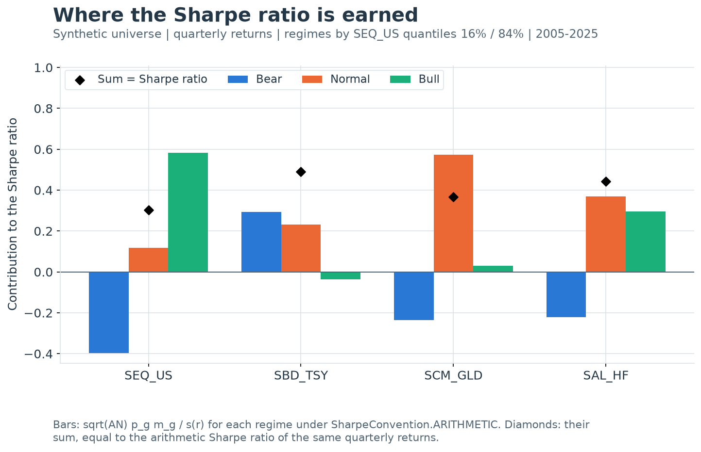
The exhibit classifies quarters by the 16% and 84% quantiles of synthetic US equity returns and plots \(\mathrm{SR}_g\) for four assets under SharpeConvention.ARITHMETIC. The diamonds are the sums, and each equals the asset’s quarterly arithmetic Sharpe ratio, as the proposition requires. Equity earns −0.40 in Bear quarters and +0.58 in Bull quarters, for a total of 0.30. Treasuries earn +0.29 of their 0.49 in Bear quarters: the profile of a crisis hedge. Gold and the hedge-fund index lose in Bear quarters and earn most of their totals in Normal quarters, so their similar totals of 0.37 and 0.44 come from different regime profiles.

The per-annum convention

The default SharpeConvention.PA reports per-annum regime returns that add up to the table’s per-annum return, and divides them by the table volatility.

Definition. Let \(R_{\mathrm{pa}}\) be the table’s PerfStat.PA_RETURN: the compound return \((P_{\mathrm{end}}/P_{\mathrm{start}})^{1/Y}-1\) between the asset’s native first and last observations, with \(Y\) in years of 365.25 days, or the total return when \(Y\le 1\). With \(x_g=\mathrm{AN}\,p_g m_g\) built from mean simple returns,

\[\begin{split} \begin{aligned} C_g&=e^{x_g}-1, \qquad \Delta=R_{\mathrm{pa}}-\sum_g C_g,\\ \tilde C_g&=C_g+p_g\,\Delta, \qquad \mathrm{SR}^{\mathrm{pa}}_g=\frac{\tilde C_g}{\hat\sigma_{\mathrm{ann}}}, \qquad \hat\sigma_{\mathrm{ann}}=\sqrt{\mathrm{AN}_{\mathrm{vol}}}\;s(v). \end{aligned} \end{split}\]

Here \(v_t\) are the PerfParams.return_type returns (log by default) on freq_vol (month-ends by default), and \(\hat\sigma_{\mathrm{ann}}\) is the PerfStat.VOL column.

Identity (per-annum additivity). \(\sum_g\tilde C_g=R_{\mathrm{pa}}\) and \(\sum_g\mathrm{SR}^{\mathrm{pa}}_g=R_{\mathrm{pa}}/\hat\sigma_{\mathrm{ann}}\).

Proof. \(\sum_g\tilde C_g=\sum_g C_g+\Delta\sum_g p_g=\sum_g C_g+\Delta=R_{\mathrm{pa}}\), because the frequencies sum to one. Divide by the common \(\hat\sigma_{\mathrm{ann}}\). \(\square\)

The additivity holds by construction, so it carries no information; the content is in how the residual is allocated. qis allocates \(\Delta\) in proportion to \(p_g\). The packaged Sharpe note described an equal split, \(\tilde C_g=C_g+\Delta/G\), which also restores the total but is not what the code computes.

Proposition (anatomy of the residual). Suppose the native endpoints lie on the regime grid and \(T/Y=\mathrm{AN}\), and write \(X=\sum_g x_g=\mathrm{AN}\,\bar r\). Then

\[ \Delta=\big(e^{\mathrm{AN}\,\bar\ell}-e^{X}\big)+\sum_{g<h}x_g\,x_h+O\big(\max_g\lvert x_g\rvert^3\big). \]

Proof. \(\log(1+R_{\mathrm{pa}})=Y^{-1}\sum_t\ell_t=\mathrm{AN}\,\bar\ell\), so \(R_{\mathrm{pa}}-(e^{X}-1)=e^{\mathrm{AN}\bar\ell}-e^{X}\). Expanding the exponentials to second order, \((e^{X}-1)-\sum_g(e^{x_g}-1)=\tfrac12\big(X^2-\sum_g x_g^2\big)+O(\lvert x\rvert^3) =\sum_{g<h}x_g x_h+O(\lvert x\rvert^3)\). Add the two pieces. \(\square\)

The first term is the volatility drag: \(\ell_t\approx r_t-r_t^2/2\), so it is close to \(-e^{X}\,\mathrm{AN}\,T^{-1}\sum_t r_t^2/2\), negative and of the order of half the annualised variance. The second is the sum of cross-products of the linear contributions; it is negative when the product of a negative Bear and a positive Bull contribution dominates, as it does for an equity-like benchmark. For the benchmark of the worked example, \(\Delta=-2.80\%\), of which \(-1.90\%\) is drag and \(-0.90\%\) cross-products.

Insight

The drag accrues where squared returns are large, which is the Bear and Bull tails, but the \(p_g\) allocation charges the residual by time spent, so the Normal regime absorbs 65% of it. In the log decomposition each term \(\mathrm{AN}\,p_g m^{\ell}_g\) carries the drag of its own periods, because \(\ell_t\approx r_t-r_t^2/2\) period by period, and the terms add up to \(\mathrm{AN}\,\bar\ell=\log(1+R_{\mathrm{pa}})\). In the worked example 78% of the benchmark’s drag accrues in the 35% of quarters labelled Bear or Bull, and its Normal contribution is 1.1% under the \(p_g\) patch against 2.5%, in log units, under the log decomposition.

The per-annum Sharpe contributions add up to \(R_{\mathrm{pa}}/\hat\sigma_{\mathrm{ann}}\). That equals PerfStat.SHARPE_RF0 only when the native endpoints lie on the freq_vol grid, because SHARPE_RF0 divides a per-annum return taken between complete freq_vol boundaries.

Pitfall

The per-annum branch mixes grids and return bases: quarterly simple-return contributions on the numerator, the volatility of monthly log returns in the denominator. The resulting bars are neither the arithmetic nor the log decomposition, and they differ from both by the volatility drag. Use SharpeConvention.ARITHMETIC or SharpeConvention.LOG when the regime bars must be an exact decomposition of a Sharpe ratio computed on one series.

Linear benchmark exposure

Proposition (beta propagation). Fit \(r_t=\hat\alpha+\hat\beta\,r_{b,t}+\hat\varepsilon_t\) by OLS with an intercept on the classified dates, and let \(\bar\varepsilon_g\) be the mean residual in regime \(g\). Then

\[ m_g=\hat\alpha+\hat\beta\,m_{b,g}+\bar\varepsilon_g, \qquad \sum_g p_g\,\bar\varepsilon_g=0, \qquad \mathrm{SR}_g=\frac{\sqrt{\mathrm{AN}}\,p_g\big(\hat\alpha+\hat\beta\,m_{b,g}+\bar\varepsilon_g\big)}{s(r)}, \]

where \(m_{b,g}\) is the benchmark’s own conditional mean.

Proof. Average the fitted identity over \(\mathcal{T}_g\). With an intercept, OLS residuals sum to zero over the sample, and \(\sum_g p_g\bar\varepsilon_g=T^{-1}\sum_t\hat\varepsilon_t\). \(\square\)

A regime profile therefore has three parts: alpha, spread over the regimes by time; beta, a scaled copy of the benchmark’s regime means; and \(\bar\varepsilon_g\), which is zero on average and captures what a straight line misses. A negative beta produces a positive Bear contribution with no skill in timing. Convexity, a payoff that gains in both tails, appears as \(\bar\varepsilon_{\mathrm{Bear}}>0\) and \(\bar\varepsilon_{\mathrm{Bull}}>0\) with \(\bar\varepsilon_{\mathrm{Normal}}<0\).

Sampling error of a contribution

Proposition. Condition on the labels, suppose the returns in regime \(g\) are independent with variance \(\sigma_g^2\), treat \(s(r)\) as fixed, and let the sample span \(Y=T/\mathrm{AN}\) years. Then

\[ \operatorname{se}(\mathrm{SR}_g)=\frac{\sqrt{\mathrm{AN}}\,p_g\,\sigma_g}{\sqrt{T_g}\;s(r)}=\sqrt{\frac{p_g}{Y}}\;\frac{\sigma_g}{s(r)} . \]

Proof. \(\operatorname{Var}(m_g)=\sigma_g^2/T_g\), and \(\mathrm{SR}_g\) is \(m_g\) times the constant \(\sqrt{\mathrm{AN}}\,p_g/s(r)\). Substitute \(T_g=p_gT=p_g\,\mathrm{AN}\,Y\). \(\square\)

For a Bear regime with \(p_g=0.175\) over ten years, \(\sqrt{p_g/Y}=0.13\): a Bear contribution carries a standard error of about 0.13 times the ratio of within-regime to total volatility. For comparison, the standard error of a full-sample Sharpe ratio is about \(\sqrt{1/Y}=0.32\) over ten years under IID returns (Lo, 2002). The formula ignores the randomness of the labels and of \(s(r)\), so it understates the uncertainty.

Worked example

The example builds ten years of monthly returns from a fixed seed: a benchmark with a monthly mean of 0.7% and volatility of 4.5%, and a hedge that returns 0.3% a month, has a beta of \(-0.30\) to the benchmark and 1.5% of idiosyncratic volatility. The classifier resamples the month-end prices to 41 quarter-end dates, 2014-12-31 to 2024-12-31, and so 40 quarterly returns. These are synthetic inputs, not market data.

The first block checks the classification. The 40 quarters split 7, 26 and 7, so \(p_g=(0.175,\,0.65,\,0.175)\). The benchmark’s conditional quarterly means are −12.62%, 1.11% and 15.38%; the hedge’s are 4.75%, 1.41% and −3.62%. The block recomputes the quarterly returns by compounding three monthly returns with numpy and the frequencies and means with a direct pd.qcut and groupby.

import numpy as np
import pandas as pd
import qis

rng = np.random.default_rng(20260725)
n_months = 120
bench = 0.007 + 0.045 * rng.standard_normal(n_months)
hedge = 0.003 - 0.30 * bench + 0.015 * rng.standard_normal(n_months)
monthly = np.column_stack([bench, hedge])
dates = pd.date_range('2014-12-31', periods=n_months + 1, freq='ME')
growth = np.vstack([np.ones((1, 2)), np.cumprod(1.0 + monthly, axis=0)])
prices = pd.DataFrame(100.0 * growth, index=dates, columns=['Benchmark', 'Hedge'])

classifier = qis.BenchmarkReturnsQuantilesRegime()  # freq='QE', edges at 0.16 and 0.84
sampled = classifier.compute_sampled_returns_with_regime_id(prices=prices, benchmark='Benchmark')

# independent quarterly returns: compound three monthly returns
quarterly = (1.0 + monthly).reshape(40, 3, 2).prod(axis=1) - 1.0
np.testing.assert_allclose(sampled[['Benchmark', 'Hedge']].iloc[1:], quarterly, atol=1e-14)
assert pd.isna(sampled['regime'].iloc[0])  # the first grid date has no return

# p_g and m_g from qis against a direct qcut and groupby
means, freqs = qis.compute_mean_freq_regimes(sampled)
q_returns = pd.DataFrame(quarterly, index=sampled.index[1:], columns=['Benchmark', 'Hedge'])
labels = pd.qcut(q_returns['Benchmark'], q=[0.0, 0.16, 0.84, 1.0],
                 labels=['Bear', 'Normal', 'Bull'])
direct_freqs = labels.value_counts(normalize=True).reindex(['Bear', 'Normal', 'Bull'])
np.testing.assert_allclose(freqs, direct_freqs, atol=1e-15)
np.testing.assert_allclose(freqs, [7 / 40, 26 / 40, 7 / 40], atol=1e-15)
np.testing.assert_allclose(means, q_returns.groupby(labels, observed=False).mean(), atol=1e-15)
np.testing.assert_allclose(means['Benchmark'], [-0.1262, 0.0111, 0.1538], atol=5e-5)
np.testing.assert_allclose(means['Hedge'], [0.0475, 0.0141, -0.0362], atol=5e-5)

Under SharpeConvention.ARITHMETIC the regime table’s Sharpe contributions of the hedge are 0.430 (Bear), 0.472 (Normal) and −0.327 (Bull). They add up to 0.575, the arithmetic Sharpe ratio \(2\,\bar r/s(r)\) of the 40 quarterly returns; the benchmark’s add up to 0.248. The table’s SHARPE_ARITH column, computed on month-end returns, is 0.588 for the hedge and 0.265 for the benchmark: a different number, on a different grid. The log decomposition adds up to the quarterly log Sharpe ratios, 0.156 and 0.542.

arith = qis.PerfParams(sharpe_convention=qis.SharpeConvention.ARITHMETIC)
table, regime_datas = classifier.compute_regimes_pa_perf_table(
    prices=prices, benchmark='Benchmark', perf_params=arith)
sharpe = regime_datas[qis.RegimeData.REGIME_SHARPE]

q_std = quarterly.std(axis=0, ddof=1)
sr_quarterly = np.sqrt(4.0) * quarterly.mean(axis=0) / q_std
np.testing.assert_allclose(sharpe.sum(axis=1), sr_quarterly, atol=1e-14)
np.testing.assert_allclose(sharpe, 2.0 * means.T.to_numpy() * freqs.to_numpy() / q_std[:, None],
                           atol=1e-14)
np.testing.assert_allclose(sr_quarterly, [0.2475, 0.5745], atol=5e-5)
np.testing.assert_allclose(sharpe.loc['Hedge'], [0.4297, 0.4719, -0.3271], atol=5e-5)
np.testing.assert_allclose(sharpe.loc['Benchmark'], [-0.4533, 0.1482, 0.5527], atol=5e-5)

# the table's SHARPE_ARITH is estimated on freq_vol='ME', not on the regime grid
sr_monthly = np.sqrt(12.0) * monthly.mean(axis=0) / monthly.std(axis=0, ddof=1)
np.testing.assert_allclose(table[qis.PerfStat.SHARPE_ARITH.to_str()], sr_monthly, atol=1e-14)
np.testing.assert_allclose(sr_monthly, [0.2655, 0.5882], atol=5e-5)

# the returns-level counterpart (internal helper) reproduces the table branch
from qis.perfstats.regime_classifier import compute_regime_sharpe_decomposition
standalone = compute_regime_sharpe_decomposition(returns=q_returns,
                                                 benchmark_returns=q_returns['Benchmark'], af=4.0)
np.testing.assert_allclose(standalone[sharpe.columns], sharpe, atol=1e-14)

# LOG: the same identity on log(1 + r)
log_params = qis.PerfParams(sharpe_convention=qis.SharpeConvention.LOG)
_, log_datas = classifier.compute_regimes_pa_perf_table(
    prices=prices, benchmark='Benchmark', perf_params=log_params)
log_q = np.log1p(quarterly)
sr_log = 2.0 * log_q.mean(axis=0) / log_q.std(axis=0, ddof=1)
np.testing.assert_allclose(log_datas[qis.RegimeData.REGIME_SHARPE].sum(axis=1), sr_log,
                           atol=1e-14)
np.testing.assert_allclose(sr_log, [0.1565, 0.5420], atol=5e-5)

The hedge’s regime profile is almost entirely linear. The quarterly OLS gives \(\hat\alpha=1.44\%\) a quarter and \(\hat\beta=-0.276\), the table’s Beta column. The Bear mean of 4.75% is \(1.44\%\) of alpha plus \(3.48\%\) of beta times the benchmark’s −12.62%, less a residual of 0.17%. Conditional on the labels, the standard errors of the three contributions are 0.117, 0.201 and 0.076: the Bear contribution of 0.43 is large relative to its error, the Normal one of 0.47 much less so.

beta, alpha = np.polyfit(quarterly[:, 0], quarterly[:, 1], deg=1)
np.testing.assert_allclose(beta, table.loc['Hedge', qis.PerfStat.BETA.to_str()], atol=1e-12)
residual_means = means['Hedge'] - (alpha + beta * means['Benchmark'])
np.testing.assert_allclose([alpha, beta], [0.0144, -0.2758], atol=5e-5)
np.testing.assert_allclose(residual_means, [-0.0017, 0.0027, -0.0082], atol=5e-5)
np.testing.assert_allclose((freqs * residual_means).sum(), 0.0, atol=1e-15)

# conditional standard errors of the contributions: sqrt(AN) p_g sigma_g / (sqrt(T_g) s(r))
within_std = q_returns['Hedge'].groupby(labels, observed=False).std()
se = 2.0 * freqs * within_std / (np.sqrt(40 * freqs) * q_returns['Hedge'].std())
np.testing.assert_allclose(se, np.sqrt(freqs / 10.0) * within_std / q_returns['Hedge'].std())
np.testing.assert_allclose(se, [0.1168, 0.2011, 0.0759], atol=5e-5)

Under the default per-annum convention the benchmark’s per-annum return is 3.04%. The compounded regime returns \(C_g\) are −8.45%, 2.93% and 11.37%, which add up to 5.84%, so \(\Delta=-2.80\%\): −1.90% of volatility drag and −0.90% of cross-products. Allocated by \(p_g\), the patched regime returns are −8.94%, 1.11% and 10.88%; an equal split would give −9.39%, 2.00% and 10.43%. Divided by the monthly log-return volatility of 16.40%, they give per-annum Sharpe contributions of −0.545, 0.068 and 0.663, which add up to SHARPE_RF0, 0.186, because the history starts and ends on month-ends. The log decomposition of the per-annum return, in log units, is −9.45%, 2.49% and 9.96%. The block also checks that the classifier honours additive_pa_returns_to_pa_total=False, which returns the unpatched \(C_g\), and that PerfStat.BEAR_AVG and its analogues select the table’s average columns.

pa_table, pa_datas = classifier.compute_regimes_pa_perf_table(
    prices=prices, benchmark='Benchmark', perf_params=qis.PerfParams())  # SharpeConvention.PA
years = (dates[-1] - dates[0]).days / 365.25
r_pa = ((prices.iloc[-1] / prices.iloc[0]) ** (1.0 / years) - 1.0).to_numpy()
np.testing.assert_allclose(pa_table[qis.PerfStat.PA_RETURN.to_str()], r_pa, atol=1e-14)

x = 4.0 * means.T.to_numpy() * freqs.to_numpy()  # rows: assets, columns: regimes
c_g = np.expm1(x)
delta = r_pa - c_g.sum(axis=1)
patched = c_g + delta[:, None] * freqs.to_numpy()
np.testing.assert_allclose(pa_datas[qis.RegimeData.REGIME_PA], patched, atol=1e-14)
np.testing.assert_allclose(pa_datas[qis.RegimeData.REGIME_PA].sum(axis=1), r_pa, atol=1e-14)
np.testing.assert_allclose(c_g[0], [-0.0845, 0.0293, 0.1137], atol=5e-5)
np.testing.assert_allclose(patched[0], [-0.0894, 0.0111, 0.1088], atol=5e-5)
np.testing.assert_allclose(c_g[0] + delta[0] / 3.0, [-0.0939, 0.0200, 0.1043], atol=5e-5)
# the classifier passes the patch switch on: False returns the unpatched C_g
_, raw_datas = classifier.compute_regimes_pa_perf_table(
    prices=prices, benchmark='Benchmark', perf_params=qis.PerfParams(),
    additive_pa_returns_to_pa_total=False)
np.testing.assert_allclose(raw_datas[qis.RegimeData.REGIME_PA], c_g, atol=1e-14)
# the regime members select the table's columns
averages = pa_table[[stat.to_str() for stat in (qis.PerfStat.BEAR_AVG, qis.PerfStat.NORMAL_AVG,
                                                 qis.PerfStat.BULL_AVG)]]
np.testing.assert_allclose(averages, means.T, atol=1e-15)

# anatomy of the residual: volatility drag plus cross-products of the contributions
drag = r_pa - np.expm1(x.sum(axis=1))
cross = (x.sum(axis=1) ** 2 - (x ** 2).sum(axis=1)) / 2.0
np.testing.assert_allclose([delta[0], drag[0], cross[0]], [-0.0280, -0.0190, -0.0090], atol=5e-5)
np.testing.assert_allclose(delta, drag + cross, atol=2e-4)

# per-annum Sharpe contributions divide by the monthly log-return volatility
vol = np.sqrt(12.0) * np.log1p(monthly).std(axis=0, ddof=1)
np.testing.assert_allclose(pa_table[qis.PerfStat.VOL.to_str()], vol, atol=1e-14)
pa_sharpe = pa_datas[qis.RegimeData.REGIME_SHARPE]
np.testing.assert_allclose(pa_sharpe, patched / vol[:, None], atol=1e-14)
np.testing.assert_allclose(pa_sharpe.sum(axis=1), pa_table[qis.PerfStat.SHARPE_RF0.to_str()],
                           atol=1e-14)
np.testing.assert_allclose(pa_sharpe.loc['Benchmark'], [-0.5453, 0.0676, 0.6633], atol=5e-5)

# the log decomposition allocates the drag where it accrues
log_means_b = pd.Series(log_q[:, 0], index=q_returns.index).groupby(labels, observed=False).mean()
log_contrib = 4.0 * freqs * log_means_b
np.testing.assert_allclose(log_contrib, [-0.0945, 0.0249, 0.0996], atol=5e-5)
np.testing.assert_allclose(log_contrib.sum(), np.log1p(r_pa[0]), atol=1e-4)
log_drag = log_contrib.to_numpy() - x[0]  # AN p_g (m_g^log - m_g)
np.testing.assert_allclose((log_drag[0] + log_drag[2]) / log_drag.sum(), 0.78, atol=5e-3)

The last block shows the two sampling caveats and checks the conditioning bias of the interpretation section. Classifying the first five years alone relabels two of those twenty quarters (2016-06-30 and 2018-12-31, Bull on the short sample and Normal on the full one). A history cut to 2015-02-15 to 2024-11-15 starts and ends with one-month stubs; the first stub, March 2015 alone, returns −8.74% and is classified Bear against full quarters. Finally, a million draws of a bivariate normal with correlation 0.5 give a correlation of about 0.25 in the Bear band and 0.30 in the Normal band, as the conditioning-bias proposition predicts.

first_half = classifier.compute_sampled_returns_with_regime_id(
    prices=prices.loc[:'2019-12-31'], benchmark='Benchmark')
short_labels = first_half['regime'].iloc[1:].astype(str)
full_labels = sampled['regime'].loc[short_labels.index].astype(str)
relabelled = short_labels.index[short_labels != full_labels]
assert list(relabelled) == [pd.Timestamp('2016-06-30'), pd.Timestamp('2018-12-31')]

stubbed = classifier.compute_sampled_returns_with_regime_id(
    prices=prices.loc['2015-02-15':'2024-11-15'], benchmark='Benchmark')
assert stubbed.index[0] == pd.Timestamp('2015-02-28')
assert stubbed.index[-1] == pd.Timestamp('2024-10-31')
np.testing.assert_allclose(stubbed['Benchmark'].iloc[1], monthly[2, 0], atol=1e-14)
np.testing.assert_allclose(monthly[2, 0], -0.0874, atol=5e-5)
assert stubbed['regime'].iloc[1] == 'Bear'

# conditioning bias: constant correlation 0.5, measured within the return bands
from scipy.stats import norm, truncnorm
draws = np.random.default_rng(1999).standard_normal((1_000_000, 2))
x_b, x_a = draws[:, 0], 0.5 * draws[:, 0] + np.sqrt(0.75) * draws[:, 1]
lower, upper = np.quantile(x_b, [0.16, 0.84])
bear, normal = x_b <= lower, (x_b > lower) & (x_b <= upper)
cut = norm.ppf(0.16)
theta = np.array([truncnorm(-np.inf, cut).var(), truncnorm(cut, -cut).var()])
predicted = 0.5 / np.sqrt(0.25 + 0.75 / theta)
np.testing.assert_allclose(theta, [0.20, 0.29], atol=5e-3)
np.testing.assert_allclose(predicted, [0.25, 0.30], atol=5e-3)
simulated = [np.corrcoef(x_b[mask], x_a[mask])[0, 1] for mask in (bear, normal)]
np.testing.assert_allclose(simulated, predicted, atol=0.01)

The quantile rule reproduces the pd.qcut labels of the first block. On six returns with a tie at the median, the median edge is 2 and all three returns equal to it fall in the lower half. A benchmark with five zero returns and one positive return cannot fill three bands: the 16% and 84% edges are 0 and 0.2, and the error reports two occupied bands of three.

from qis.utils.quantile_buckets import (EmptyQuantileBucketError, classify_quantile_buckets,
                                        compute_bucket_codes, compute_quantile_edges)

rule = classify_quantile_buckets(q_returns['Benchmark'], q=[0.0, 0.16, 0.84, 1.0],
                                 labels=['Bear', 'Normal', 'Bull'])
assert (rule.astype(str) == labels.astype(str)).all()

ties = np.array([1.0, 2.0, 2.0, 2.0, 3.0, 4.0])
np.testing.assert_allclose(compute_quantile_edges(ties, q=2), [2.0])
np.testing.assert_array_equal(compute_bucket_codes(ties, q=2), [0, 0, 0, 0, 1, 1])

degenerate = np.array([0.0, 0.0, 0.0, 0.0, 0.0, 1.0])
np.testing.assert_allclose(compute_quantile_edges(degenerate, q=[0.0, 0.16, 0.84, 1.0]), [0.0, 0.2])
try:
    compute_bucket_codes(degenerate, q=[0.0, 0.16, 0.84, 1.0])
except EmptyQuantileBucketError as error:
    assert (error.num_occupied, error.num_buckets) == (2, 3)
else:
    raise AssertionError('a degenerate benchmark must be rejected')

Implementation in qis

Quantity	Formula	qis entry point
Return-quantile regimes	Bear, Normal, Bull at \(\hat Q_b(0.16)\), \(\hat Q_b(0.84)\)	qis.BenchmarkReturnsQuantilesRegime(freq='QE', q=None), method compute_sampled_returns_with_regime_id
Sign regimes	Negative if \(r_{b,t}<0\), else Positive	qis.BenchmarkReturnsPositiveNegativeRegime(freq='QE')
Volatility regimes	q equal-count buckets of within-period realised volatility	qis.BenchmarkVolsQuantilesRegime(freq='QE', q=4)
Frequencies and means	\(p_g=T_g/T\), \(m_g\)	qis.compute_mean_freq_regimes
Regime averages and contributions	\(m_g\); \(C_g=e^{x_g}-1\), or \(x_g\) with is_report_pa_returns=False	qis.compute_regime_avg(freq=...)
Patched per-annum returns	\(\tilde C_g=C_g+p_g\Delta\)	additive_pa_returns_to_pa_total=True (default) in the classifiers’ compute_regimes_pa_perf_table and in qis.compute_regimes_pa_perf_table_from_sampled_returns
Benchmark display row	\(m_g\) in place of \(\tilde C_g\) for the benchmark, display only	is_use_benchmark_means=True in qis.compute_regimes_pa_perf_table_from_sampled_returns
Arithmetic and log contributions	\(\mathrm{SR}_g\), \(\mathrm{SR}^{\ell}_g\)	PerfParams(sharpe_convention=SharpeConvention.ARITHMETIC) or LOG
Per-annum contributions	\(\mathrm{SR}^{\mathrm{pa}}_g=\tilde C_g/\hat\sigma_{\mathrm{ann}}\)	PerfParams(), SharpeConvention.PA
Regime table	all of the above plus the risk-adjusted table	qis.RegimeClassifier.compute_regimes_pa_perf_table, qis.compute_bnb_regimes_pa_perf_table
Returns-level contributions	\(\mathrm{SR}_g\), \(\mathrm{SR}^{\ell}_g\) and their total	internal qis.perfstats.regime_classifier.compute_regime_sharpe_decomposition(returns, benchmark_returns, af)
Panels	\(m_g\); \(\tilde C_g\); \(\mathrm{SR}_g\) in the selected convention	qis.RegimeData.REGIME_AVG, REGIME_PA, REGIME_SHARPE
Table columns	\(m_g\), \(\tilde C_g\), \(\mathrm{SR}_g\)	PerfStat.BEAR_AVG ('Bear Average'), PerfStat.BEAR_PA, PerfStat.BEAR_SHARPE, and the Normal and Bull analogues; qis.SD_PERF_COLUMNS carries the three Sharpe columns
Exhibits	stacked regime bars; boxplots; shading	qis.plot_regime_data, qis.plot_regime_boxplot, qis.add_bnb_regime_shadows
Quantile rule	edges, right-closed buckets, ties in the lower bucket	qis.utils.quantile_buckets.classify_quantile_buckets, compute_bucket_codes, compute_quantile_edges
Nulls, premia, regime betas	Gaussian null of each contribution and the convexity premium	qis.regimes; see the convexity premium

The classification and tables are in regime_classifier.py, the exhibits in regime_data.py, and RegimeData, SharpeConvention, PerfParams and the regime PerfStat members in config.py. API pages: regime table, quantile classifier and regime exhibit.

Implementation contracts that affect the numbers:

• Call path. compute_bnb_regimes_pa_perf_table builds a BenchmarkReturnsQuantilesRegime from freq, return_type and q, unless a regime_classifier keyword supplies one, and returns only the table. The classifier’s compute_regimes_pa_perf_table classifies, then calls compute_regimes_pa_perf_table_from_sampled_returns and returns the table together with a dictionary keyed by RegimeData.REGIME_AVG, REGIME_PA and REGIME_SHARPE.

• Frequency and convention. \(\mathrm{AN}\) is get_annualization_factor(freq) of the classifier’s freq. The Sharpe convention is perf_params.sharpe_convention; perf_params=None means SharpeConvention.PA, and the attached table then infers its frequency from the price index.

• Options on the classifier path. The classifiers’ compute_regimes_pa_perf_table accept additive_pa_returns_to_pa_total (default True) and pass it on, so additive_pa_returns_to_pa_total=False reports the unpatched \(C_g\). The base RegimeClassifier.compute_regimes_pa_perf_table also passes its remaining keywords on, among them is_report_pa_returns=False for the linear contributions \(x_g\). The classifiers’ own methods fix is_use_benchmark_means=False; that option is set on compute_regimes_pa_perf_table_from_sampled_returns called directly. Earlier versions accepted additive_pa_returns_to_pa_total on the classifier path but did not forward it.

• is_use_benchmark_means=True replaces the benchmark row of the P.a. columns by its periodic conditional means \(m_g\), a display choice. The regime Sharpe values are computed before the substitution, so the benchmark’s per-annum Sharpe contributions stay \(\tilde C_g/\hat\sigma_{\mathrm{ann}}\). Earlier versions divided the displayed periodic means by the annualised volatility.

• Missing values. \(p_g\) counts benchmark-classified dates, \(m_g\) averages the asset’s observed returns and \(s(r)\) uses all of them, so the table’s contributions add up exactly only when the asset is observed on the classified dates and on no others. The internal returns-level function computes every moment per asset over the dates where both the asset and the benchmark are observed, and is exact for any gap pattern. An empty regime has no mean: the table and the internal function both report a missing contribution, and the plot’s totals and the function’s total skip it, since an empty regime contributes nothing to the mean.

• Return type. The classifier’s return_type sets the returns behind \(m_g\) and \(C_g\). With the default ReturnTypes.RELATIVE they are simple returns: the ARITHMETIC branch uses them and the LOG branch takes \(\log(1+r)\). With ReturnTypes.LOG they are log returns: the LOG branch uses them as they are and the ARITHMETIC branch converts them with \(e^{\ell}-1\), so each convention decomposes its own Sharpe ratio whatever the classifier’s basis.

• Column labels. The average columns are labelled 'Bear Average', 'Normal Average' and 'Bull Average', the labels of the PerfStat.BEAR_AVG family; the P.a. and Sharpe columns match PerfStat.BEAR_PA and PerfStat.BEAR_SHARPE. Every regime member therefore selects a column, for example in qis.plot_ra_perf_scatter. The labels do not carry the Sharpe convention; state it with the table.

• Exhibits. plot_regime_data passes prices, benchmark and perf_params through to the classifier and stacks the chosen RegimeData panel; the bar totals are the row sums. add_bnb_regime_shadows shades each grid interval \((t-1,t]\) in the colour of the regime of the period ending at \(t\), which matches the return timing.

Interpretation and limitations

Crisis beta and risk-premia alpha

Sepp (2019) reads the regime profile as a classification of strategies. A strategy whose Bear contribution is positive earns part of its Sharpe ratio when the benchmark falls: crisis beta, the profile of trend-following managers. A strategy that earns its Sharpe ratio in the Normal regime and loses in the Bear regime is paid a premium for bearing crisis risk: risk-premia alpha, the profile of many alternative risk premia. An equity-like benchmark has a negative Bear, a small Normal and a large Bull contribution, as in the worked example.

The beta-propagation proposition sharpens the reading. A positive Bear contribution can come from a negative beta, which a short benchmark position delivers at the cost of a negative Bull contribution, or from convexity, \(\bar\varepsilon_{\mathrm{Bear}}>0\) together with \(\bar\varepsilon_{\mathrm{Bull}}>0\), which pays in the Bear regime without giving up the Bull regime. The hedge of the worked example is the first kind: its regime means are the line \(\hat\alpha+\hat\beta\,m_{b,g}\) to within 0.9% a quarter.

The convexity premium turns this distinction into one number per asset. Under a jointly Gaussian null each regime contribution is a closed form in the Sharpe ratio and the correlation with the benchmark, and the excess of the realised Bear contribution over its null, net of the benchmark’s own departure, is the Bear-regime residual mean in Sharpe units. The premium adds up across a portfolio with risk weights, which is how Sepp and Kastenholz (2026) rank overlays of a principal portfolio.

Conditional correlations and the conditioning bias

The chapter’s statistics are conditional means. Conditional correlations and betas estimated within a regime behave differently, because selecting periods by the value of one variable changes that variable’s variance.

Proposition (conditioning bias). Let \((r_b,r)\) be bivariate normal with correlation \(\rho\), and let \(\mathcal{A}\) be an event defined by \(r_b\) alone, with variance ratio \(\theta_{\mathcal{A}}=\operatorname{Var}(r_b\mid\mathcal{A})/\operatorname{Var}(r_b)\). Then

\[ \rho_{\mathcal{A}}=\frac{\rho}{\sqrt{\rho^2+(1-\rho^2)/\theta_{\mathcal{A}}}} , \]

so \(\lvert\rho_{\mathcal{A}}\rvert<\lvert\rho\rvert\) when \(\theta_{\mathcal{A}}<1\) and \(\lvert\rho_{\mathcal{A}}\rvert>\lvert\rho\rvert\) when \(\theta_{\mathcal{A}}>1\).

Proof. Standardise both returns and write \(r=\rho r_b+\sqrt{1-\rho^2}\,u\) with \(u\) standard normal and independent of \(r_b\), so conditioning on \(\mathcal{A}\) leaves \(u\) unchanged. Then \(\operatorname{Cov}(r_b,r\mid\mathcal{A})=\rho\,\theta_{\mathcal{A}}\) and \(\operatorname{Var}(r\mid\mathcal{A})=\rho^2\theta_{\mathcal{A}}+1-\rho^2\). Divide the covariance by the square root of the product of the variances. \(\square\)

This is the pitfall of Boyer, Gibson and Loretan (1999): a constant-correlation model produces “correlation breakdowns” in subsamples selected by the size of one return. Truncating a standard normal below \(\Phi^{-1}(0.16)=-0.994\) leaves a variance ratio of about 0.20, and the central band about 0.29. With \(\rho=0.5\) the within-regime correlations are about 0.25 in the Bear band and 0.30 in the Normal band, although nothing has changed. Conditioning on large absolute returns, \(\theta_{\mathcal{A}}>1\), inflates correlation instead. Longin and Solnik (2001) account for the bias by comparing exceedance correlations, the correlations of returns that jointly exceed a threshold, with their values under normality, and model the tails with extreme value theory. Under normality the exceedance correlation goes to zero as the threshold moves into the tails; they find that it does not for large negative returns, and that equity-market correlation rises in bear markets but not in bull markets.

Insight

Conditional means do not suffer the variance-truncation bias. Under the model of the proposition, \(\mathbb{E}[r\mid\mathcal{A}]-\mathbb{E}[r]=\beta\,\big(\mathbb{E}[r_b\mid\mathcal{A}]-\mathbb{E}[r_b]\big)\) for every \(\mathcal{A}\), with the full-sample \(\beta\). This is why a mean-based regime profile is interpretable with a constant beta while a within-regime beta or correlation needs the correction above before it can be read as a change in dependence.

Model-based regimes

The qis regimes are labels on observed benchmark returns, not a model. A regime-switching model instead treats the regime as a latent Markov state with its own means, volatilities and correlations, estimated by maximum likelihood with the filter described in Hamilton (1994). Ang and Bekaert (2002) use such a model for international asset allocation; they find a high-volatility, high-correlation bear regime in which international diversification still pays. A model gives state probabilities, persistence and transition probabilities that labels cannot; its filtered probabilities use only past data and can drive a backtest, while its smoothed probabilities use the full sample, like the qis labels. qis does not implement regime-switching estimation.

Limitations

• Look-ahead. Full-sample edges and contemporaneous labels make every regime statistic descriptive. Do not feed the labels, or statistics conditioned on them, into a backtest.

• Few observations in the tails. Ten years of quarters leave seven Bear and seven Bull observations. The conditional standard error is about \(\sqrt{p_g/Y}\) times the ratio of within-regime to total volatility, before accounting for label uncertainty.

• Stubs. An off-grid history adds a short first and last period, classified against full quarters and annualised as quarters. Trim prices to quarter-ends for a clean quarterly sample.

• Conventions differ. Arithmetic, log and per-annum regime bars are three different numbers on the same data. In the worked example the benchmark totals are 0.248, 0.156 and 0.186. State the convention with the exhibit: plot_regime_data’s default title, Conditional Sharpe ratio, does not name it. No convention deducts cash.

• Benchmark dependence. The regime is a property of the benchmark, and a different benchmark gives a different partition. A benchmark back-padded with constant prices adds zero returns that crowd the Normal band, and raises ValueError if they collapse a quantile edge; clip the panel to the benchmark’s live window first.

See also

• The convexity premium and smart diversification

• Sharpe ratios: conventions and inference

• The performance-statistic catalogue: every PerfStat column

• Alpha, beta and benchmark-relative performance

• Covariance, correlation and principal components

• Notation and conventions

• Reporting frequency and annualisation

• Factsheets and reporting

• Bibliography

References

1. Sepp, A. (2019). Trend-Following CTAs vs Alternative Risk-Premia: Crisis Beta vs Risk-Premia Alpha. The Hedge Fund Journal. Article. Uses the Bear, Normal and Bull decomposition of Sharpe ratios to separate crisis beta from risk-premia alpha.

2. Sharpe, W. F. (1994). The Sharpe Ratio. The Journal of Portfolio Management, 21(1), 49–58. Author’s copy. The arithmetic Sharpe ratio of periodic returns that the additive decomposition splits.

3. Lo, A. W. (2002). The Statistics of Sharpe Ratios. Financial Analysts Journal, 58(4), 36–52. DOI: 10.2469/faj.v58.n4.2453. The sampling error of a full-sample Sharpe ratio used as the comparison for regime contributions.

4. Boyer, B. H., Gibson, M. S., and Loretan, M. (1999). Pitfalls in tests for changes in correlations. Federal Reserve Board, International Finance Discussion Papers 597. PDF. The conditioning bias of correlations estimated in subsamples.

5. Longin, F., and Solnik, B. (2001). Extreme Correlation of International Equity Markets. The Journal of Finance, 56(2), 649–676. DOI: 10.1111/0022-1082.00340. Exceedance correlations and the asymmetry between bear and bull markets.

6. Ang, A., and Bekaert, G. (2002). International Asset Allocation with Regime Shifts. The Review of Financial Studies, 15(4), 1137–1187. DOI: 10.1093/rfs/15.4.1137. The regime-switching alternative to descriptive labels.

7. Hamilton, J. D. (1994). Time Series Analysis. Princeton University Press. The filter and smoother of Markov-switching models.

8. Sepp, A., and Kastenholz, M. (2026). The Convexity Premium of Portfolio Overlays. Journal of Investment Management, forthcoming. The Gaussian null of the regime contributions and the convexity premium.

9. Sepp, A. qis: Performance analytics, portfolio backtesting, risk analysis, and factsheet reporting in Python. Software citation metadata.