The convexity premium and smart diversification

Author: Artur Sepp

Implemented in qis — Quantitative Investment Strategies. Software citation: CITATION.cff.

The regime decomposition splits a Sharpe ratio into what an asset earned in the Bear, Normal and Bull periods of a benchmark. This chapter asks how much of a Bear contribution correlation alone explains. When the asset and the benchmark are jointly Gaussian, every regime contribution is a closed form in the asset’s Sharpe ratio and its correlation with the benchmark; the realised Bear contribution less that null is the convexity premium of Sepp and Kastenholz (2026). The premium adds up across the constituents of a portfolio with risk weights, which makes it the measure of what an overlay adds to a principal portfolio in the periods when the principal falls. The subpackage qis.regimes computes the nulls, the premia, their bootstrap intervals, regime betas and regime-mixture moments, and qis.SmartDiversificationReport draws the curves that trade the Bear contribution against the Sharpe ratio.

Overview

A positive Bear contribution can be bought in two ways. A short benchmark position earns it through negative correlation and pays for it with a negative Bull contribution. A convex payoff, such as a long straddle or a trend-following strategy that adapts within the period, earns it without giving up the Bull regime. The beta-propagation proposition of the regime chapter separates the two with the mean regression residual of each regime; this chapter turns that separation into one number per asset and shows how it aggregates.

The calculation has four steps:

1. Classify. Label each period Bear, Normal or Bull by the quantiles of the benchmark’s return, as the regime chapter does: the one-sigma cut at 16% and 84% by default.

2. Decompose. Compute each asset’s arithmetic regime contributions, which add up to its Sharpe ratio on the regime grid.

3. Compare with the null. Compute the contribution a jointly Gaussian asset with the same Sharpe ratio and correlation would have, and subtract it. The difference in the lowest bucket is the convexity premium; net of the benchmark’s own departure from the null it is the benchmark-adjusted premium.

4. Aggregate. A portfolio’s Bear contribution is its null plus the risk-weighted sum of its constituents’ premia. Mixing a principal portfolio with one overlay traces a curve of Bear contribution against Sharpe ratio: the smart-diversification curve.

The chapter proves the null, identifies what the premium measures, derives the aggregation identity and the closed-form blend frontier, and treats regime betas and the regime-mixture covariance, which carry the same non-linearity into risk models. Like the regime labels, every statistic here is descriptive: the quantile edges use the whole sample.

Inputs, notation, and assumptions

Convention	This article
Return basis	Simple total returns on the regime grid, as in the arithmetic regime decomposition; no cash is deducted, so pass excess-return NAVs for excess statistics
Sampling grid	The regime grid of the sampled frame: quarter-ends from BenchmarkReturnsQuantilesRegime(freq='QE'), or any periodic returns through create_sampled_returns_with_regime_id; the report’s per-annum statistics use PerfParams(freq='ME')
Annualisation	\(\mathrm{AN}\) of the regime grid, passed as af (4 for quarters): \(\sqrt{\mathrm{AN}}\) in contributions, loadings and \(\kappa\); ann_vol is \(\sqrt{\mathrm{AN}}\,s(r)\)
Mean adjustment	Regime means are raw; \(s(r)\) is demeaned with ddof=1; correlations are Pearson; regression intercepts are estimated and then discarded
Timing	Descriptive and full sample: quantile edges use the whole history; the bootstraps reclassify every resample; the regime-time EWMA is seeded with each stream’s full-sample mean
Output units	Contributions, nulls and premia in annualised Sharpe units; <tail>_return_pa in decimal per year; betas dimensionless; covariances annualised
qis default	compute_regime_premium_table(sampled, benchmark, af, q=None, nu=None): one-sigma cut [0.0, 0.16, 0.84, 1.0], Gaussian null; compute_regime_premium_bootstrap(block_size=8, n_boot=2000, seed=7, ci=0.95)

Symbol or input	Meaning	Units and convention
\(r_t\), \(r_{b,t}\)	Asset and benchmark simple return on the regime grid	Decimal per period
\(g\), \(G\)	Regime index and number of regimes, from the lowest benchmark bucket up	Bear, Normal, Bull: \(G=3\); the code writes \(s\)
\(q_0<q_1<\dots<q_G\)	Partition probabilities, \(q_0=0\), \(q_G=1\)	q; one-sigma cut by default
\(\pi_g\)	Partition probability of regime \(g\), \(q_g-q_{g-1}\)	0.16, 0.68, 0.16 on the one-sigma cut
\(p_g\)	Realised frequency of regime \(g\)	\(T_g/T\), as in the regime chapter
\(m_g\), \(m_{b,g}\)	Mean return of the asset and of the benchmark in regime \(g\)	Decimal per period
\(\mathrm{SR}\), \(\mathrm{SR}_b\)	Arithmetic Sharpe ratios \(\sqrt{\mathrm{AN}}\,\bar r/s(r)\) on the regime grid	Annualised
\(\mathrm{SR}_g\)	Regime contribution \(\sqrt{\mathrm{AN}}\,p_g m_g/s(r)\)	Adds up to \(\mathrm{SR}\) over \(g\)
\(\rho\)	Correlation of the asset with the benchmark	Sample Pearson correlation
\(Z\)	Unit-variance benchmark shock, \((r_b-\mu_b)/\sigma_b\)	Gaussian or Student-t margin
\(z_g\)	Edge of regime \(g\) in units of \(Z\), \(z_0=-\infty\), \(z_G=+\infty\)	Quantile \(q_g\) of the margin
\(\phi\), \(\Phi\)	Standard normal density and distribution function
\(k_g\)	Null loading of regime \(g\), \(\sqrt{\mathrm{AN}}\,\mathbb{E}[Z\,1\{z_{g-1}<Z\le z_g\}]\)	Sums to zero over \(g\)
\(\kappa\)	Bull loading of a symmetric three-bucket cut, the Bear one being \(-\kappa\)	0.487 quarterly, 0.843 monthly
\(\nu\)	Degrees of freedom of a Student-t null	\(\nu>2\); calibrated as \(4+6/\text{kurtosis}\)
\(\mathrm{CP}\), \(\mathrm{CP}_b\)	Convexity premium of the asset and of the benchmark	Lowest bucket, annualised Sharpe units
\(\mathrm{CP}^{*}\)	Benchmark-adjusted premium \(\mathrm{CP}-\rho\,\mathrm{CP}_b\)	Zero for the benchmark
\(\bar\varepsilon_g\)	Mean OLS residual of \(r\) on \(r_b\) in regime \(g\)	As in the regime chapter
\(x\)	Overlay weight of a blend \((1-x)\,\)benchmark \(+\,x\,\)overlay	0 to 1
\(\sigma_p\), \(\rho_p\), \(\mathrm{SR}_p\)	Volatility, benchmark correlation and Sharpe ratio of a portfolio	Annualised
\(\beta_{i,g}\)	Regime beta of asset \(i\) on the benchmark in regime \(g\)	OLS slope within the regime
\(v_i\)	Per-period residual variance of asset \(i\)	idio_vars

Inputs are the frame a regime classifier returns: periodic returns with a categorical regime column, built by BenchmarkReturnsQuantilesRegime.compute_sampled_returns_with_regime_id from prices or by qis.regimes.create_sampled_returns_with_regime_id from returns. Every function of qis.regimes works for any partition of the benchmark’s returns: three buckets are labelled Bear, Normal and Bull, other counts Q1 to Qn, and the premium always refers to the lowest bucket. The subpackage is imported explicitly, from qis.regimes import ...; its names are not exported from qis. Classification follows the one quantile rule of qis in qis.utils.quantile_buckets, described in the regime chapter: linear-interpolation edges, buckets closed on the right, and a return equal to an interior edge in the lower bucket.

Methodology

The Gaussian null of the regime contributions

Proposition (Gaussian null, Sepp and Kastenholz 2026). Let the asset and the benchmark returns of a period be jointly normal with means \(\mu\), \(\mu_b\), volatilities \(\sigma\), \(\sigma_b\) and correlation \(\rho\), and let regime \(g\) be the event \(z_{g-1}<Z\le z_g\) with \(z_g=\Phi^{-1}(q_g)\). The population regime contribution \(\mathrm{SR}_g=\sqrt{\mathrm{AN}}\,\mathbb{E}[r\,1\{g\}]/\sigma\) is

\[ \mathrm{SR}_g=\pi_g\,\mathrm{SR}+\rho\,k_g, \qquad k_g=\sqrt{\mathrm{AN}}\,\big(\phi(z_{g-1})-\phi(z_g)\big), \]

with \(\mathrm{SR}=\sqrt{\mathrm{AN}}\,\mu/\sigma\) and \(\phi(\pm\infty)=0\).

Proof. For a jointly normal pair the conditional mean is linear, \(\mathbb{E}[r\mid Z]=\mu+\rho\,\sigma Z\), so \(\mathbb{E}[r\,1\{g\}]=\mu\,\pi_g+\rho\,\sigma\,\mathbb{E}[Z\,1\{g\}]\). Because \(\phi'(z)=-z\,\phi(z)\), \(\int_a^b z\,\phi(z)\,dz=\phi(a)-\phi(b)\). Divide by \(\sigma\) and multiply by \(\sqrt{\mathrm{AN}}\). \(\square\)

The loadings telescope, \(\sum_g k_g=\sqrt{\mathrm{AN}}\,(\phi(-\infty)-\phi(+\infty))=0\), so the null contributions add up to \(\mathrm{SR}\) for any partition. On a symmetric three-bucket cut the loadings are \(-\kappa\), \(0\) and \(\kappa\) with

\[ \kappa=\sqrt{\mathrm{AN}}\;\phi\big(\Phi^{-1}(1-\pi_1)\big), \]

which is 0.487 for quarterly and 0.843 for monthly regimes on the one-sigma cut. The Bear null is \(\pi_1\mathrm{SR}-\kappa\rho\). The proof uses only two properties: the conditional mean of the asset is linear in the benchmark, and the benchmark’s margin is Gaussian. Any asset whose excess over its linear projection has zero mean in every bucket sits on the null, whatever its own distribution.

Insight

In these coordinates one unit of correlation costs \(\kappa\) of Bear contribution and one unit of Sharpe ratio buys \(\pi_1\). At quarterly frequency \(\kappa/\pi_1=3.04\): lowering the correlation with the benchmark by 0.1 improves the Bear contribution as much as raising the Sharpe ratio by 0.30. On monthly regimes the ratio is 5.27. Diversifying away from the benchmark is the cheap route to a better Bear contribution; the premium measures what an asset earns beyond it.

Proposition (Student-t null). Let the pair be jointly Student-t with \(\nu>2\) degrees of freedom, so that \(Z=\sqrt{(\nu-2)/\nu}\,W\) with \(W\) Student-t of density \(f_\nu\), and let \(w_g\) be the quantile \(q_g\) of \(W\). The conditional mean is still linear, and

\[ k_g=\sqrt{\mathrm{AN}}\,\sqrt{\frac{\nu-2}{\nu}}\,\big(h_\nu(w_{g-1})-h_\nu(w_g)\big), \qquad h_\nu(w)=\frac{\nu+w^2}{\nu-1}\,f_\nu(w). \]

Proof. Elliptical distributions have linear conditional means, so the first proof carries over with \(\mathbb{E}[Z\,1\{g\}]\). Write \(f_\nu(w)=c_\nu(1+w^2/\nu)^{-(\nu+1)/2}\). Then \((\nu+w^2)f_\nu(w)=\nu\,c_\nu(1+w^2/\nu)^{-(\nu-1)/2}\), whose derivative is \(-(\nu-1)\,w\,f_\nu(w)\), so \(\int_a^b w\,f_\nu(w)\,dw=h_\nu(a)-h_\nu(b)\). The factor \(\sqrt{(\nu-2)/\nu}\) converts \(W\) to unit variance. \(\square\)

A unit-variance Student-t margin puts more mass near the centre and in the far tails. At the one-sigma cut its \(\kappa\) is therefore below the Gaussian value, 0.475 against 0.487 for \(\nu=5\), while at 5% tails it is above, 0.224 against 0.206; both converge to the Gaussian value as \(\nu\) grows. calibrate_student_t_nu matches the benchmark’s sample excess kurtosis \(K\), which is \(6/(\nu-4)\) for a Student-t, by \(\nu=4+6/K\) with a floor of 4.5, and returns None for \(K\le0\), when the Gaussian null is the tighter benchmark.

The convexity premium

Definition (convexity premium). With \(\mathrm{SR}_1\) the realised contribution of the lowest bucket, \(\pi_1\) its partition probability and \(k_1\) its null loading,

\[ \mathrm{CP}=\mathrm{SR}_1-\big(\pi_1\,\mathrm{SR}+\rho\,k_1\big), \qquad \mathrm{CP}^{*}=\mathrm{CP}-\rho\,\mathrm{CP}_b, \]

where \(\mathrm{CP}_b\) is the benchmark’s own premium, with \(\rho=1\). On the one-sigma cut \(\mathrm{CP}=\mathrm{SR}_{\mathrm{Bear}}-(0.16\,\mathrm{SR}-\kappa\rho)\).

The realised contribution uses the realised frequency \(p_1\) and the null the partition probability \(\pi_1\), which differ by the rounding of the quantile position: 14 of 83 quarters is 0.169 rather than 0.16. The benchmark itself has a premium when its lowest bucket is shallower or deeper than a Gaussian’s, and every correlated asset inherits that departure in proportion to \(\rho\). The next result makes this precise.

Proposition (what the premium measures). Let \(r=\alpha+\beta r_b+\varepsilon\) be the population linear projection, with \(\mathbb{E}[\varepsilon]=0\) and \(\operatorname{Cov}(\varepsilon,r_b)=0\), and let the buckets be the population quantile buckets of \(r_b\) with any margin. Then

\[ \mathrm{CP}=\rho\,\mathrm{CP}_b+\frac{\sqrt{\mathrm{AN}}\,\pi_1\,\mathbb{E}[\varepsilon\mid 1]}{\sigma}, \qquad \mathrm{CP}^{*}=\frac{\sqrt{\mathrm{AN}}\,\pi_1\,\mathbb{E}[\varepsilon\mid 1]}{\sigma}. \]

Proof. Write \(r_b=\mu_b+\sigma_b Z\). Since \(\alpha+\beta\mu_b=\mu\) and \(\beta\sigma_b=\rho\sigma\), \(\mathbb{E}[r\,1\{1\}]=\mu\,\pi_1+\rho\,\sigma\,\mathbb{E}[Z\,1\{1\}] +\mathbb{E}[\varepsilon\,1\{1\}]\). For the benchmark, with \(\rho=1\) and no residual, \(\mathrm{SR}_{b,1}=\pi_1\mathrm{SR}_b+\sqrt{\mathrm{AN}}\,\mathbb{E}[Z\,1\{1\}]\). Substituting, \(\mathrm{SR}_1=\pi_1\mathrm{SR}+\rho(\mathrm{SR}_{b,1}-\pi_1\mathrm{SR}_b) +\sqrt{\mathrm{AN}}\,\pi_1\mathbb{E}[\varepsilon\mid1]/\sigma\). Subtract the null \(\pi_1\mathrm{SR}+\rho k_1\) and recognise \(\mathrm{CP}_b=\mathrm{SR}_{b,1}-\pi_1\mathrm{SR}_b-k_1\). \(\square\)

The premium has two sources: the shape of the benchmark’s own lower tail, carried at the asset’s correlation, and the lowest-bucket mean of the part of the asset’s return that no straight line in the benchmark explains. The benchmark-adjusted premium keeps only the second. It is zero whenever the conditional mean is linear, as under the Gaussian and Student-t nulls, and it is positive for a payoff that is convex in the benchmark.

Identity (the benchmark-adjusted premium in sample). Fit \(r_t=\hat\alpha+\hat\beta r_{b,t}+\hat\varepsilon_t\) by OLS with an intercept over the classified periods, let \(\bar\varepsilon_1\) be the mean residual of the lowest bucket and \(\hat\rho\) the sample correlation. Then

\[ \mathrm{CP}^{*}=\frac{\sqrt{\mathrm{AN}}\,p_1\,\bar\varepsilon_1}{s(r)} +(p_1-\pi_1)\big(\mathrm{SR}-\hat\rho\,\mathrm{SR}_b\big). \]

Proof. From the regime chapter, \(m_1=\hat\alpha+\hat\beta m_{b,1}+\bar\varepsilon_1\), with \(\hat\alpha=\bar r-\hat\beta\bar r_b\) and \(\hat\beta=\hat\rho\,s(r)/s(r_b)\). Multiplying by \(\sqrt{\mathrm{AN}}\,p_1/s(r)\) gives \(\mathrm{SR}_1=p_1\mathrm{SR}+\hat\rho(\mathrm{SR}_{b,1}-p_1\mathrm{SR}_b) +\sqrt{\mathrm{AN}}\,p_1\bar\varepsilon_1/s(r)\). Subtract the null \(\pi_1\mathrm{SR}+\hat\rho k_1\), then \(\hat\rho\) times \(\mathrm{CP}_b=\mathrm{SR}_{b,1}-\pi_1\mathrm{SR}_b-k_1\). \(\square\)

The in-sample identity is the population result plus a frequency-mismatch term, which vanishes when the lowest bucket holds exactly \(\pi_1 T\) periods. It ties the premium to the residual means \(\bar\varepsilon_g\) of the beta-propagation proposition: the benchmark-adjusted premium is the Bear-regime residual mean expressed as a contribution to the Sharpe ratio.

compute_regime_premium_bootstrap measures the sampling error of the premium. It resamples each asset jointly with the benchmark by the stationary block bootstrap of Politis and Romano (1994), with geometric blocks of mean length 8 periods, and reclassifies the regimes inside every resample, so the interval includes the uncertainty of the quantile edges. A resample repeats observations, which puts returns on the edges; the quantile rule assigns them to the lower bucket.

Aggregation across a portfolio

Proposition (aggregation identity, Sepp and Kastenholz 2026). Let a portfolio hold constant weights \(w_i\) on the regime grid, \(r_{p,t}=\sum_i w_i r_{i,t}\), and let every asset and the portfolio be classified by the same benchmark. With risk weights \(\omega_i=w_i\,\sigma_i/\sigma_p\),

\[ \mathrm{SR}_{p,g}=\sum_i\omega_i\,\mathrm{SR}_{i,g}, \qquad \mathrm{SR}_p=\sum_i\omega_i\,\mathrm{SR}_i, \qquad \rho_p=\sum_i\omega_i\,\rho_i, \qquad \mathrm{CP}_p=\sum_i\omega_i\,\mathrm{CP}_i, \]

and hence \(\mathrm{SR}_{p,1}=\pi_1\mathrm{SR}_p+\rho_p k_1+\sum_i\omega_i\,\mathrm{CP}_i\), which on the one-sigma cut reads \(\pi_1\mathrm{SR}_p-\kappa\rho_p+\sum_i\omega_i\mathrm{CP}_i\).

Proof. The regime means, the mean and the covariance with the benchmark are linear in the weights: \(m_{p,g}=\sum_i w_i m_{i,g}\) and \(\operatorname{Cov}(r_p,r_b)=\sum_i w_i\,\rho_i\,\sigma_i\sigma_b\). Dividing by \(\sigma_p\), or by \(\sigma_p\sigma_b\), turns each into the stated risk-weighted sum, with the regime frequencies common to all assets. The null \(\pi_1\mathrm{SR}+\rho k_1\) is linear in \((\mathrm{SR},\rho)\), so the premia aggregate with the same weights. \(\square\)

The identity holds exactly in sample, for the realised contributions and the sample moments, provided the portfolio’s returns are the weighted sums of the constituents’ returns on the regime grid: a portfolio rebalanced at the start of every regime period. The risk weights do not add up to one; their sum \(\sum_i w_i\sigma_i/\sigma_p\) is the diversification ratio of Choueifaty and Coignard (2008), at least one for a long-only portfolio. Diversification multiplies the risk-weighted average premium by that ratio, exactly as it multiplies the average Sharpe ratio.

The overlay blend frontier

A funded blend holds \(1-x\) in the benchmark and \(x\) in one overlay \(a\). Applying the aggregation identity to the two assets gives the frontier in closed form.

Proposition (blend frontier). With the overlay’s Sharpe ratio \(\mathrm{SR}_a\), volatility \(\sigma_a\), correlation \(\rho\) and premium \(\mathrm{CP}_a\), and the benchmark’s \(\mathrm{SR}_b\), \(\sigma_b\) and \(\mathrm{CP}_b\),

\[\begin{split} \begin{aligned} \sigma_p^2&=(1-x)^2\sigma_b^2+x^2\sigma_a^2+2x(1-x)\rho\,\sigma_a\sigma_b, \qquad \mathrm{SR}_p=\frac{(1-x)\,\mathrm{SR}_b\,\sigma_b+x\,\mathrm{SR}_a\,\sigma_a}{\sigma_p},\\ \rho_p&=\frac{(1-x)\,\sigma_b+x\,\rho\,\sigma_a}{\sigma_p}, \qquad \mathrm{SR}_{p,1}=\pi_1\mathrm{SR}_p+\rho_p k_1 +\frac{x\,\sigma_a\,\mathrm{CP}_a+(1-x)\,\sigma_b\,\mathrm{CP}_b}{\sigma_p}. \end{aligned} \end{split}\]

Proof. The first two lines are the variance and mean of a two-asset portfolio. The benchmark’s correlation with itself is one, so \(\rho_p\) and the Bear contribution follow from the aggregation identity with \(\omega=\big((1-x)\sigma_b,\,x\sigma_a\big)/\sigma_p\). \(\square\)

compute_overlay_blend_frontier evaluates the frontier with \(\mathrm{CP}_b=0\), a benchmark on its null. For a benchmark with a premium of its own, add \((1-x)\,\sigma_b\,\mathrm{CP}_b/\sigma_p\) to its bear_sharpe column; the worked example shows that the result then equals the realised contributions of the blends to rounding error.

Proposition (uncorrelated overlay). For \(\rho=0\) and positive Sharpe ratios the frontier peaks at \(x^{*}=(\mathrm{SR}_a/\sigma_a)/(\mathrm{SR}_a/\sigma_a+\mathrm{SR}_b/\sigma_b)\) with \(\mathrm{SR}_p=\sqrt{\mathrm{SR}_a^2+\mathrm{SR}_b^2}\).

Proof. With a diagonal covariance the maximum Sharpe ratio over all weights is \(\sqrt{\mu^{\top}\Sigma^{-1}\mu}=\sqrt{\mathrm{SR}_a^2+\mathrm{SR}_b^2}\), attained at weights proportional to \(\mu_i/\sigma_i^2=\mathrm{SR}_i/\sigma_i\), which normalised to a sum of one give \(x^{*}\) in \((0,1)\). \(\square\)

Open full-resolution preview.

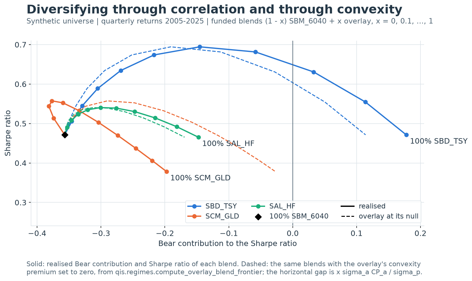
The exhibit mixes the synthetic 60/40 benchmark with three overlays in funded blends and plots each blend’s Bear contribution against its Sharpe ratio, from the benchmark alone (the diamond) to the overlay alone. Solid curves are realised; dashed curves are the same blends with the overlay moved onto its null, \(\mathrm{CP}_a=0\), so the horizontal gap is \(x\,\sigma_a\,\mathrm{CP}_a/\sigma_p\). Treasuries diversify through correlation, \(-0.08\), and a premium of \(+0.06\): a 60% blend lifts the Sharpe ratio from 0.47 to 0.69 and the Bear contribution from \(-0.36\) to \(-0.15\). Gold’s correlation is also low, 0.18, but its premium of \(-0.17\) bends its curve to the left: gold falls more in Bear quarters than its correlation implies, and every blend with up to 40% gold has a worse Bear contribution than the benchmark alone. The hedge-fund index sits close to its null.

The smart-diversification exhibit

qis.SmartDiversificationReport draws the same curves from NAVs. For each overlay, create_overlay_portfolio_curve backtests eleven mixes of the principal portfolio and the overlay with qis.backtest_model_portfolio, rebalanced at rebalancing_freq (quarter-ends by default), with overlay weights from zero to max_overlay_weight. Two mixing rules are available:

• is_principal_weight_fixed=True (default) keeps the principal at principal_weight and adds the overlay on top, weights \((1, x)\). The mix is levered, which suits an overlay that is an unfunded, excess-return strategy such as a futures programme.

• is_principal_weight_fixed=False funds the overlay from the principal, weights \((1-x, x)\): the blends of the frontier above.

compute_smart_diversification_curve reads two statistics off the mixes, by default PerfStat.BEAR_SHARPE on the x axis and PerfStat.SHARPE_RF0 on the y axis, classifying every mix against the first one, which holds no overlay and so is the principal portfolio. plot_smart_diversification_curve draws one curve per overlay, and plot_smart_diversification_scatter one point per standalone overlay with a cross-sectional fit.

The report’s statistics follow its PerfParams, PerfParams(freq='ME') by default, and hence SharpeConvention.PA: its Bear axis is the per-annum Bear contribution of the regime chapter, not the arithmetic contribution that the null and the premium use. Pass perf_params=qis.PerfParams(freq='ME', sharpe_convention=qis.SharpeConvention.ARITHMETIC) to put the curves in the coordinates of this chapter; the funded curves then match the closed-form frontier, up to the rebalancing dates discussed in the implementation notes.

Regime betas

compute_regime_betas fits, within each regime, an OLS regression of the asset on the benchmark with an intercept and keeps the slope \(\beta_{i,g}\); forcing the fit through the origin would bias it. The pooled residuals of the piecewise fit give the idiosyncratic volatility.

Proposition (selection on the benchmark leaves the slope unbiased). If \(r=\alpha+\beta r_b+\varepsilon\) with \(\mathbb{E}[\varepsilon\mid r_b]=0\), then for every event \(\mathcal{A}\) defined by \(r_b\) alone the population slope within \(\mathcal{A}\) is \(\beta\).

Proof. \(\operatorname{Cov}(r,r_b\mid\mathcal{A})=\beta\operatorname{Var}(r_b\mid\mathcal{A}) +\operatorname{Cov}(\varepsilon,r_b\mid\mathcal{A})\), and the last term is zero because \(\mathbb{E}[\varepsilon\mid r_b]=0\) holds on \(\mathcal{A}\). Divide by \(\operatorname{Var}(r_b\mid\mathcal{A})\). \(\square\)

Under a linear conditional mean every regime beta equals the total beta, so their spread measures non-linearity; a convex payoff has betas that rise from the Bear to the Bull regime. This is the contrast with the conditioning bias of correlations: the same selection that leaves the slope unbiased shrinks a within-regime correlation, because it shrinks the benchmark’s variance but not the residual’s. compute_regime_betas_bootstrap resamples whole rows of the panel with the stationary block bootstrap, which keeps the cross-section, reclassifies each resample and re-estimates, and reports the standard deviation of the resampled betas.

compute_regime_ewm_betas and compute_regime_ewm_avg run EWMA recursions over each regime’s own stream of periods rather than calendar time. A calendar-time EWMA discounts a crisis by its calendar age, so the Bear moments of a long sample are set by whichever Bear periods are recent; in regime time the last Bear period carries the most weight among Bear periods however long ago it occurred. Both recursions are seeded with the stream’s full-sample mean (InitType.MEAN), so at a span far longer than the stream they return the equal-weighted estimates, and inside a backtest they must be evaluated on the data known at each decision date.

Regime-mixture moments

Proposition (regime-mixture covariance). Let asset \(i\) follow \(r_i=a_i+\beta_{i,g}\,r_b+\varepsilon_i\) in regime \(g\), with a regime-independent intercept \(a_i\) and residuals independent across assets and of the benchmark, with variance \(v_i\). With \(m_{b,g}\) and \(S_g\) the benchmark’s mean and second moment in regime \(g\),

\[ \operatorname{Cov}(r_i,r_j)=\sum_g\pi_g\,\beta_{i,g}\beta_{j,g}\,S_g -\Big(\sum_g\pi_g\,\beta_{i,g}\,m_{b,g}\Big)\Big(\sum_g\pi_g\,\beta_{j,g}\,m_{b,g}\Big) +1\{i=j\}\,v_i . \]

Proof. By total expectation, \(\mathbb{E}[r_ir_j]=\sum_g\pi_g\,\mathbb{E}[r_ir_j\mid g]\) and \(\mathbb{E}[r_i]=\sum_g\pi_g\,\mathbb{E}[r_i\mid g]\). The intercept terms cancel in \(\mathbb{E}[r_ir_j]-\mathbb{E}[r_i]\mathbb{E}[r_j]\) because \(a_i\) does not depend on \(g\), and the residuals contribute \(v_i\) on the diagonal only. \(\square\)

compute_regime_mixture_covar evaluates the formula and multiplies by \(\mathrm{AN}\); the benchmark enters as an asset with unit betas and zero residual. With equal betas in every regime the first two terms reduce to \(\beta_i\beta_j\operatorname{Var}(r_b)\), the single-factor covariance. The regime intercepts are discarded, as in the regime betas, and residual correlations are not modelled.

Identity (Gaussian regime moments). For a standard normal \(Z\) and a bucket \(a<Z\le b\) with probability \(\pi\),

\[ \mathbb{E}[Z\mid a<Z\le b]=\frac{\phi(a)-\phi(b)}{\pi}, \qquad \mathbb{E}[Z^2\mid a<Z\le b]=1+\frac{a\,\phi(a)-b\,\phi(b)}{\pi}. \]

Proof. The first is the truncated first moment of the Gaussian null. For the second, integrate by parts: \(\int_a^b z^2\phi(z)\,dz=\big[-z\,\phi(z)\big]_a^b+\int_a^b\phi(z)\,dz\). \(\square\)

On the one-sigma cut the Bear mean is \(-1.521\) volatilities, the tail variances are 0.200 and the Normal variance 0.288 squared volatilities, the variance ratios behind the conditioning bias of the regime chapter. compute_gaussian_regime_moments scales them by the benchmark’s periodic volatility and mean, which gives the regime inputs of the mixture covariance from one volatility, with nothing else estimated.

Worked example

The first block checks the null loadings. The quarterly and monthly \(\kappa\) of the one-sigma cut are 0.4866 and 0.8429, the loadings of the symmetric cut are exactly antisymmetric, and the loadings of an asymmetric partition, \([0,0.05,0.5,1]\), equal the integrated truncated moments: \(-0.206\), \(-0.592\) and \(0.798\). For a Student-t null with \(\nu=5\), \(\kappa\) is 0.475 at the one-sigma cut and 0.224 at 5% tails, against Gaussian values of 0.487 and 0.206; an excess kurtosis of 1.5 calibrates \(\nu=8\).

import numpy as np
import pandas as pd
from scipy import integrate
from scipy.stats import norm
from scipy.stats import t as student_t
import qis
from qis.regimes import (calibrate_student_t_nu, compute_regime_kappa,
                         compute_regime_null_loadings)

kappa = compute_regime_kappa(af=4.0)
np.testing.assert_allclose([kappa, compute_regime_kappa(af=12.0)], [0.4866, 0.8429], atol=5e-5)
np.testing.assert_allclose(kappa, 2.0 * norm.pdf(norm.ppf(0.84)), rtol=1e-14)
loadings = compute_regime_null_loadings(af=4.0)
assert loadings['Bear'] == -loadings['Bull'] == -kappa and loadings['Normal'] == 0.0

# an asymmetric partition against quadrature of the truncated first moment
q = [0.0, 0.05, 0.5, 1.0]
edges = norm.ppf(q)
direct = [2.0 * integrate.quad(lambda z: z * norm.pdf(z), a, b)[0]
          for a, b in zip(edges[:-1], edges[1:])]
np.testing.assert_allclose(compute_regime_null_loadings(af=4.0, q=q), direct, atol=1e-9)
np.testing.assert_allclose(direct, [-0.2063, -0.5916, 0.7979], atol=5e-5)

# Student-t null: the kernel (nu + w^2) f(w) / (nu - 1), scaled to unit variance
nu = 5.0
w = student_t.ppf(0.84, df=nu)
kernel = (nu + w ** 2) / (nu - 1.0) * student_t.pdf(w, df=nu)
kappa_t = compute_regime_kappa(af=4.0, nu=nu)
np.testing.assert_allclose(kappa_t, 2.0 * kernel * np.sqrt((nu - 2.0) / nu), rtol=1e-12)
np.testing.assert_allclose([kappa_t, compute_regime_kappa(af=4.0, tail_prob=0.05),
                            compute_regime_kappa(af=4.0, tail_prob=0.05, nu=nu)],
                           [0.4753, 0.2063, 0.2239], atol=5e-5)
assert calibrate_student_t_nu(excess_kurtosis=1.5) == 8.0
assert calibrate_student_t_nu(excess_kurtosis=-0.05) is None

The second block simulates 200,000 periods of a standard normal benchmark and two assets: a linear asset, jointly Gaussian with the benchmark, with a Sharpe ratio of 0.50 and a correlation of 0.60; and a straddle that earns the benchmark’s absolute return less its mean, plus noise. The linear asset sits on its null, with a premium of \(-0.001\), and its regime betas, 0.048, 0.048 and 0.047, equal its total beta of 0.048 to sampling error. The straddle is uncorrelated with the benchmark, yet its Bear contribution exceeds the null by 0.271, and its regime betas rise from \(-0.050\) through zero to \(+0.050\): convexity in both of its signatures.

from qis.regimes import (compute_regime_betas, compute_regime_premium_table,
                         create_sampled_returns_with_regime_id)

rng = np.random.default_rng(20260725)
z = rng.standard_normal((200_000, 3))
simulated = pd.DataFrame({
    'Benchmark': z[:, 0],
    'Linear': 0.02 + 0.08 * (0.6 * z[:, 0] + 0.8 * z[:, 1]),
    'Straddle': 0.01 + 0.05 * (np.abs(z[:, 0]) - np.sqrt(2.0 / np.pi)) + 0.03 * z[:, 2],
})
sim_sampled = create_sampled_returns_with_regime_id(simulated, benchmark='Benchmark')
sim_table = compute_regime_premium_table(sim_sampled, benchmark='Benchmark', af=4.0)
np.testing.assert_allclose(sim_table.loc['Linear', ['sharpe', 'rho']], [0.50, 0.60], atol=5e-3)
assert abs(sim_table.loc['Linear', 'convexity_premium']) < 0.005
np.testing.assert_allclose(sim_table.loc['Straddle', ['rho', 'convexity_premium']],
                           [0.0, 0.271], atol=5e-3)

sim_betas = compute_regime_betas(sim_sampled, benchmark='Benchmark', af=4.0).astype(float)
regime_betas = ['beta_bear', 'beta_normal', 'beta_bull']
np.testing.assert_allclose(sim_betas.loc['Linear', regime_betas + ['beta_total']],
                           [0.0476, 0.0481, 0.0468, 0.0479], atol=5e-5)
np.testing.assert_allclose(sim_betas.loc['Straddle', regime_betas], [-0.050, 0.0, 0.050],
                           atol=1e-3)

The third block computes the premium table on the frozen synthetic universe: the 60/40 benchmark SBM_6040, US equities, Treasuries, gold and a hedge-fund index, on quarterly returns from 2005-03-31 to 2025-12-31. Starting on a quarter-end avoids a stub period, and 83 quarters split 14, 55 and 14. The benchmark’s own premium is \(+0.054\): its 14 Bear quarters average \(-5.4\%\), against \(-6.5\%\) for the lowest 16% of a Gaussian with the same mean and volatility. Equities inherit that departure at their correlation of 0.97 and have a benchmark-adjusted premium of \(-0.008\). Treasuries have \(+0.068\) and gold \(-0.180\), of which \(-0.183\) is gold’s Bear-quarter regression residual of \(-4.2\%\) a quarter expressed as a Sharpe contribution. The bootstrap standard errors of the premia are 0.026 to 0.067, and only gold’s 95% interval excludes zero.

from qis.datasets import generate_synthetic_universe
from qis.regimes import compute_regime_premium_bootstrap

universe = generate_synthetic_universe(start='2005-01-03', end='2025-12-31', seed=20260725,
                                       apply_quirks=False)
assets = ['SBM_6040', 'SEQ_US', 'SBD_TSY', 'SCM_GLD', 'SAL_HF']
prices = pd.concat([universe.benchmark_prices, universe.prices], axis=1)[assets]
prices = prices.loc['2005-03-31':]  # start on a quarter-end: no stub period
classifier = qis.BenchmarkReturnsQuantilesRegime(freq='QE')
sampled = classifier.compute_sampled_returns_with_regime_id(prices=prices, benchmark='SBM_6040')
data = sampled.dropna(subset=['regime'])
table = compute_regime_premium_table(sampled, benchmark='SBM_6040', af=4.0)
assert data['regime'].value_counts().to_dict() == {'Normal': 55, 'Bear': 14, 'Bull': 14}
np.testing.assert_allclose(table['convexity_premium'], [0.0543, 0.0449, 0.0636, -0.1703, 0.0217],
                           atol=5e-5)
np.testing.assert_allclose(table['cp_star'], [0.0, -0.0079, 0.0679, -0.1801, -0.0055], atol=5e-5)

# the benchmark's Bear quarters against the lowest 16% of a Gaussian with its mean and volatility
bear = (data['regime'].astype(str) == 'Bear').to_numpy()
b = data['SBM_6040'].to_numpy()
gaussian_bear_mean = b.mean() - norm.pdf(norm.ppf(0.16)) / 0.16 * b.std(ddof=1)
np.testing.assert_allclose([b[bear].mean(), gaussian_bear_mean], [-0.0539, -0.0655], atol=5e-5)

# the adjusted premium: the Bear-mean OLS residual plus the frequency-mismatch term
sr_b = 2.0 * b.mean() / b.std(ddof=1)
residual_part = {}
for asset in assets[1:]:
    r = data[asset].to_numpy()
    slope, intercept = np.polyfit(b, r, 1)
    residual = r - intercept - slope * b
    sr, rho = 2.0 * r.mean() / r.std(ddof=1), np.corrcoef(r, b)[0, 1]
    residual_part[asset] = 2.0 * bear.mean() * residual[bear].mean() / r.std(ddof=1)
    identity = residual_part[asset] + (bear.mean() - 0.16) * (sr - rho * sr_b)
    np.testing.assert_allclose(table.loc[asset, 'cp_star'], identity, atol=1e-12)
    if asset == 'SCM_GLD':
        np.testing.assert_allclose([residual[bear].mean(), residual_part[asset]],
                                   [-0.0422, -0.1827], atol=5e-5)

boot = compute_regime_premium_bootstrap(data[assets], benchmark='SBM_6040', af=4.0, n_boot=500)
np.testing.assert_allclose(boot['premium_se'], [0.0258, 0.0667, 0.0658, 0.0616], atol=5e-5)
assert boot.loc['SCM_GLD', 'premium_ci_high'] < 0.0 < boot.loc['SBD_TSY', 'premium_ci_high']

Open full-resolution preview.

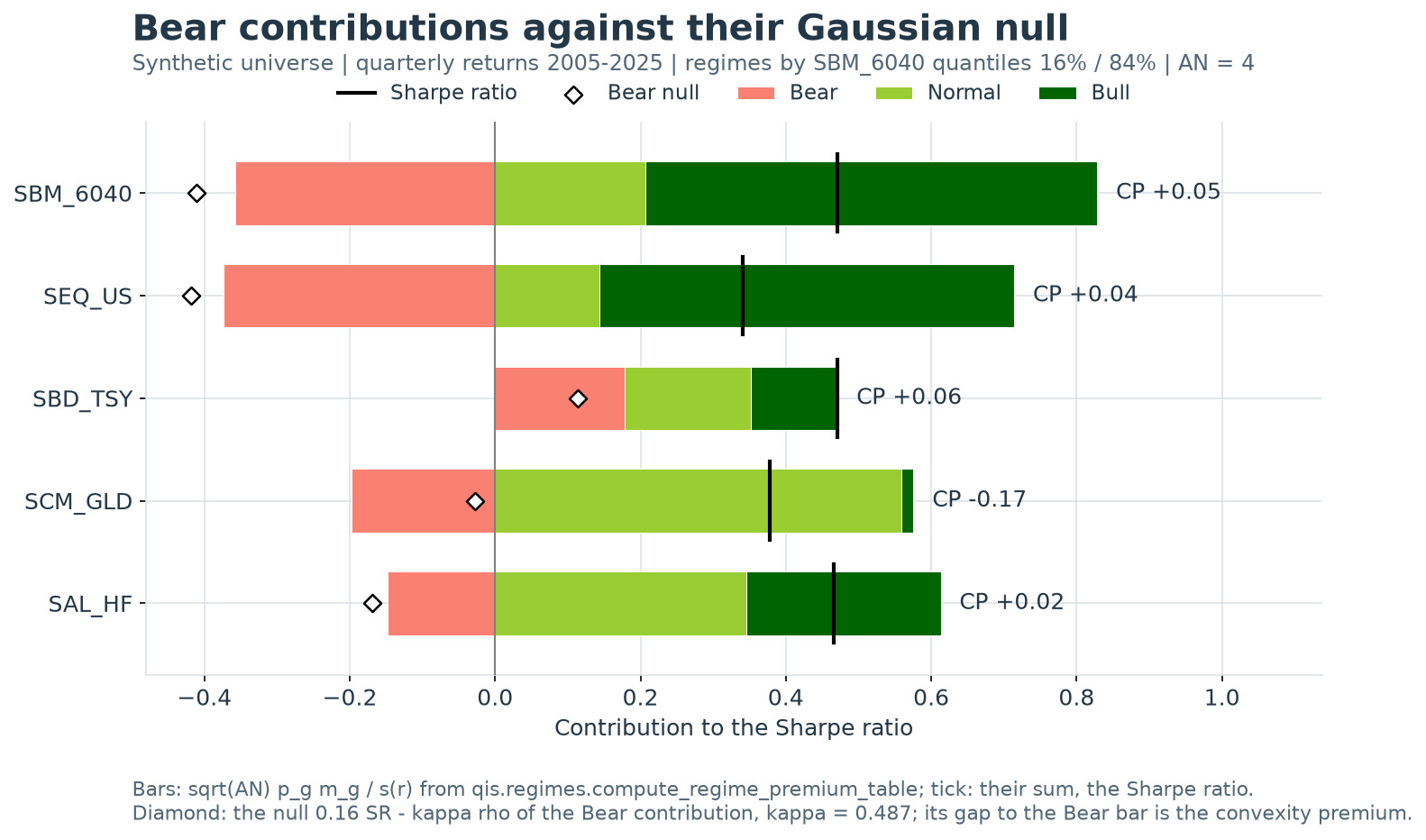
The exhibit draws the table with qis.plots.derived.regime_premium.plot_regime_sharpe_decomposition. The distance from each diamond, the Gaussian null of the Bear contribution, to the end of the Bear bar is the premium printed beside the row. The 60/40 benchmark and equities lose 0.36 and 0.37 of Sharpe ratio in Bear quarters, slightly less than their nulls. Treasuries earn 0.18, above a null of 0.11. Gold’s null is almost zero, \(-0.03\), because its correlation is low, but it loses 0.20.

The fourth block checks the aggregation identity on a constant-weight quarterly portfolio of 40% equities, 40% Treasuries, 10% gold and 10% hedge funds. Its risk weights add up to a diversification ratio of 1.58, and its premium, 0.031, is the risk-weighted sum of the constituents’ premia. It then evaluates the funded Treasury frontier in closed form: with the benchmark’s own premium added back, it reproduces the Sharpe ratios and Bear contributions of the realised blends to \(10^{-12}\). The frontier peaks at a 60% overlay with a Sharpe ratio of 0.694, and an uncorrelated overlay with equal Sharpe ratios peaks at \(\sqrt2\,\mathrm{SR}\).

from qis.regimes import compute_overlay_blend_frontier, compute_portfolio_bear_sharpe

weights = pd.Series({'SEQ_US': 0.4, 'SBD_TSY': 0.4, 'SCM_GLD': 0.1, 'SAL_HF': 0.1})
portfolio = (data[weights.index] * weights).sum(axis=1).rename('Portfolio')
extended = compute_regime_premium_table(pd.concat([data, portfolio], axis=1),
                                        benchmark='SBM_6040', af=4.0)
row, members = extended.loc['Portfolio'], extended.loc[weights.index]
risk_weights = weights * members['ann_vol'] / row['ann_vol']
aggregated = compute_portfolio_bear_sharpe(
    weights=weights.to_numpy(), vols=members['ann_vol'].to_numpy(),
    srs=members['sharpe'].to_numpy(), rhos=members['rho'].to_numpy(),
    premia=members['convexity_premium'].to_numpy(), portfolio_vol=row['ann_vol'], af=4.0)
np.testing.assert_allclose(aggregated, row['bear_sharpe'], atol=1e-12)
np.testing.assert_allclose(row['convexity_premium'],
                           (risk_weights * members['convexity_premium']).sum(), atol=1e-12)
np.testing.assert_allclose([risk_weights.sum(), row['convexity_premium']], [1.584, 0.0308],
                           atol=5e-4)

# the funded Treasury frontier against the realised blends
x = np.linspace(0.0, 1.0, 11)
b_row, a_row = table.loc['SBM_6040'], table.loc['SBD_TSY']
frontier = compute_overlay_blend_frontier(
    sr_b=b_row['sharpe'], vol_b=b_row['ann_vol'], sr_a=a_row['sharpe'], vol_a=a_row['ann_vol'],
    rho=a_row['rho'], af=4.0, premium_a=a_row['convexity_premium'], overlay_weights=x)
blends = pd.DataFrame({f'{v:.1f}': (1.0 - v) * data['SBM_6040'] + v * data['SBD_TSY'] for v in x})
realised = compute_regime_premium_table(pd.concat([data[['SBM_6040', 'regime']], blends], axis=1),
                                        benchmark='SBM_6040', af=4.0).loc[blends.columns]
benchmark_term = ((1.0 - x) * b_row['ann_vol'] / frontier['portfolio_vol'].to_numpy()
                  * b_row['convexity_premium'])
np.testing.assert_allclose(frontier['sharpe'], realised['sharpe'], atol=1e-12)
np.testing.assert_allclose(frontier['bear_sharpe'] + benchmark_term, realised['bear_sharpe'],
                           atol=1e-12)
assert np.isclose(frontier['sharpe'].idxmax(), 0.6)
np.testing.assert_allclose(realised.loc['0.6', ['sharpe', 'rho', 'bear_sharpe']],
                           [0.6944, 0.7053, -0.1455], atol=5e-5)

# gold blends: a Bear contribution below the benchmark's up to a 40% overlay
gold = pd.DataFrame({f'{v:.1f}': (1.0 - v) * data['SBM_6040'] + v * data['SCM_GLD'] for v in x})
gold_table = compute_regime_premium_table(pd.concat([data[['SBM_6040', 'regime']], gold], axis=1),
                                          benchmark='SBM_6040', af=4.0)
gold_bear = gold_table.loc[gold.columns, 'bear_sharpe']
assert list(gold_bear.index[gold_bear < b_row['bear_sharpe']]) == ['0.1', '0.2', '0.3', '0.4']

uncorrelated = compute_overlay_blend_frontier(sr_b=0.5, vol_b=0.10, sr_a=0.5, vol_a=0.06, rho=0.0,
                                              af=4.0, overlay_weights=[0.625])
np.testing.assert_allclose(uncorrelated['sharpe'], np.hypot(0.5, 0.5), rtol=1e-12)

The fifth block runs the report. With the arithmetic convention its standalone points equal the table’s Bear contributions, and its funded Treasury curve matches the realised blends to within 0.0004. Under the report’s default per-annum convention the same principal has a Bear value of \(-0.374\) rather than \(-0.357\): a different statistic. Finally, mixes built from the full synthetic history, which starts on 3 January 2005 between quarter-ends, are invested from that date: the zero-weight mix is the principal itself.

from qis.portfolio.smart_diversification import (SmartDiversificationReport,
                                                 create_overlay_portfolio_curve)

bear_column = qis.PerfStat.BEAR_SHARPE.to_str()
overlays = prices[['SBD_TSY', 'SCM_GLD', 'SAL_HF']]
arithmetic = qis.PerfParams(freq='ME', sharpe_convention=qis.SharpeConvention.ARITHMETIC)
report = SmartDiversificationReport(overlay_navs=overlays, principal_nav=prices['SBM_6040'],
                                    perf_params=arithmetic)
points = report.get_overlay_points(principal_nav=prices['SBM_6040'])
np.testing.assert_allclose(points[bear_column], table.loc[points.index, 'bear_sharpe'],
                           atol=1e-12)
curve = report.compute_smart_diversification_curve(principal_nav=prices['SBM_6040'],
                                                   overlay_nav=prices['SBD_TSY'],
                                                   is_principal_weight_fixed=False)
np.testing.assert_allclose(curve[bear_column], realised['bear_sharpe'], atol=5e-4)

default_points = SmartDiversificationReport(
    overlay_navs=overlays, principal_nav=prices['SBM_6040']).get_overlay_points(
    principal_nav=prices['SBM_6040'])
np.testing.assert_allclose(default_points.loc['SBM_6040', bear_column], -0.3738, atol=5e-5)

full_principal = universe.benchmark_prices['SBM_6040']
unaligned = create_overlay_portfolio_curve(principal_nav=full_principal,
                                           overlay_nav=universe.prices['SBD_TSY'],
                                           is_principal_weight_fixed=False)
np.testing.assert_allclose(unaligned.iloc[:, 0] / unaligned.iloc[0, 0],
                           full_principal / full_principal.iloc[0], rtol=1e-12)

The sixth block estimates regime betas. Each equals the within-regime covariance ratio. The hedge-fund index has betas of 0.05, 0.83 and 0.02 in the three regimes against a total beta of 0.42, a pattern that looks like strong non-linearity; its bootstrap standard errors, 0.74 in the Bear regime and 0.30 in the Bull, show that 14 quarters per tail cannot confirm it.

from qis.regimes import compute_regime_betas_bootstrap

betas = compute_regime_betas(sampled, benchmark='SBM_6040', af=4.0).astype(float)
labels = data['regime'].astype(str)
for asset in betas.index:
    for regime in ('Bear', 'Normal', 'Bull'):
        pair = data.loc[labels == regime, [asset, 'SBM_6040']].to_numpy()
        covariance = np.cov(pair.T)
        np.testing.assert_allclose(betas.loc[asset, f'beta_{regime.lower()}'],
                                   covariance[0, 1] / covariance[1, 1], rtol=1e-10)
np.testing.assert_allclose(betas.loc['SAL_HF', regime_betas + ['beta_total']],
                           [0.050, 0.833, 0.023, 0.424], atol=5e-4)
betas_se = compute_regime_betas_bootstrap(data[assets], benchmark='SBM_6040', af=4.0, n_boot=200)
np.testing.assert_allclose(betas_se.loc['SAL_HF', ['beta_bear_se', 'beta_bull_se']],
                           [0.736, 0.297], atol=5e-4)

The last block checks the regime moments. The Gaussian regime moments are \(-1.521\), 0 and \(+1.521\) volatilities with variances 0.200, 0.288 and 0.200; weighted by the partition probabilities they recover the benchmark’s variance exactly, and with equal regime betas the mixture covariance is the single-factor covariance. A regime-time EWMA with a span far longer than any stream returns the equal-weighted regime means; with a span of eight Bear quarters the 60/40 Bear mean is \(-5.03\%\) against the equal-weighted \(-5.39\%\).

from qis.regimes import (compute_gaussian_regime_moments, compute_regime_ewm_avg,
                         compute_regime_mixture_covar, get_regime_probabilities)

means, second = compute_gaussian_regime_moments(benchmark_vol=1.0)
np.testing.assert_allclose(means, [-1.5207, 0.0, 1.5207], atol=5e-5)
np.testing.assert_allclose(second - means ** 2, [0.1997, 0.2883, 0.1997], atol=5e-5)

s_b, m_b = data['SBM_6040'].std(), data['SBM_6040'].mean()
means_b, second_b = compute_gaussian_regime_moments(benchmark_vol=s_b, benchmark_mean=m_b)
probs = get_regime_probabilities()
np.testing.assert_allclose((probs * second_b).sum() - (probs * means_b).sum() ** 2, s_b ** 2,
                           rtol=1e-12)
beta_total = betas['beta_total']
flat = pd.DataFrame({regime: beta_total for regime in probs.index})
idio = betas['idio_vol'] ** 2 / 4.0  # per-period residual variances
mixture = compute_regime_mixture_covar(flat, idio, means_b, second_b, af=4.0)
single = 4.0 * (np.outer(beta_total, beta_total) * s_b ** 2 + np.diag(idio))
np.testing.assert_allclose(mixture, single, rtol=1e-12)

long_span = compute_regime_ewm_avg(sampled, span=1e6)
regime_means = data.drop(columns='regime').groupby(data['regime'], observed=True).mean()
np.testing.assert_allclose(long_span, regime_means.reindex(long_span.index), atol=1e-9)
short_span = compute_regime_ewm_avg(sampled, span=8.0)
bear_means = [short_span.loc['Bear', 'SBM_6040'], regime_means.loc['Bear', 'SBM_6040']]
np.testing.assert_allclose(bear_means, [-0.0503, -0.0539], atol=5e-5)

Implementation in qis

Quantity	Formula	qis entry point
Partition	\(\pi_g=q_g-q_{g-1}\); ids Bear, Normal, Bull or Q1 to Qn	qis.regimes.get_partition_quantiles, get_regime_probabilities, get_regime_ids, ONE_SIGMA_QUANTILES
Sampled frame from returns	periodic returns with the benchmark-quantile regime	qis.regimes.create_sampled_returns_with_regime_id(returns, benchmark, q=None)
Null loadings	\(k_g\), Gaussian or Student-t	qis.regimes.compute_regime_null_loadings(af, q=None, nu=None)
\(\kappa\)	\(\sqrt{\mathrm{AN}}\,\phi(\Phi^{-1}(1-\pi_1))\)	qis.regimes.compute_regime_kappa(af, tail_prob=0.16, nu=None)
Student-t calibration	\(\nu=\max(4+6/K,\,4.5)\)	qis.regimes.calibrate_student_t_nu(excess_kurtosis, min_nu=4.5)
Null contributions	\(\pi_g\mathrm{SR}+\rho k_g\)	qis.regimes.compute_null_regime_contributions(sr, rho, af, q=None, nu=None)
Convexity premium	\(\mathrm{SR}_1-(\pi_1\mathrm{SR}-\kappa\rho)\)	qis.regimes.compute_convexity_premium(sr_bear, sr, rho, af)
Premium table	contributions, null, \(\mathrm{CP}\), \(\mathrm{CP}^{*}\), <tail>_return_pa	qis.regimes.compute_regime_premium_table(sampled, benchmark, af, q=None, nu=None)
Premium bootstrap	stationary blocks, reclassified	qis.regimes.compute_regime_premium_bootstrap(returns, benchmark, af, block_size=8, n_boot=2000)
Aggregation	\(\pi_1\mathrm{SR}_p-\kappa\rho_p+\sum_i\omega_i\mathrm{CP}_i\)	qis.regimes.compute_portfolio_bear_sharpe
Blend frontier	\(\sigma_p\), \(\mathrm{SR}_p\), \(\rho_p\), \(\mathrm{SR}_{p,1}\) with \(\mathrm{CP}_b=0\)	qis.regimes.compute_overlay_blend_frontier
Regime betas	within-regime OLS slopes, pooled residual volatility	qis.regimes.compute_regime_betas, compute_regime_betas_bootstrap(block_size=12)
Regime-time EWMA	EWMA over each regime’s stream, seeded at its mean	qis.regimes.compute_regime_ewm_avg, compute_regime_ewm_betas
Mixture covariance	law of total covariance times \(\mathrm{AN}\)	qis.regimes.compute_regime_mixture_covar
Gaussian regime moments	truncated normal mean and second moment	qis.regimes.compute_gaussian_regime_moments(benchmark_vol, benchmark_mean=0.0, q=None)
Exhibits	stacked contributions with null; regime-beta profiles	qis.plots.derived.regime_premium.plot_regime_sharpe_decomposition, plot_regime_beta_profiles
Smart diversification	eleven mixes, Bear contribution against Sharpe ratio	qis.SmartDiversificationReport, qis.create_overlay_portfolio_curve

The analytics are in src/qis/regimes/, the exhibits in regime_premium.py, the report in src/qis/portfolio/smart_diversification/ and the quantile rule in quantile_buckets.py. The API reference lists the explicitly imported subpackages beside the exported names.

Implementation contracts that affect the numbers:

• Moments. compute_regime_premium_table computes \(s(r)\), the regime means and the correlation over each asset’s available classified periods, \(p_g\) over all classified periods and the Sharpe ratio with compute_sharpe_arithmetic(ddof=1). On a panel without gaps its contributions equal the internal compute_regime_sharpe_decomposition and add up to sharpe.

• Frequencies. The contributions use the realised \(p_g\) and the null the partition’s \(\pi_g\). A symmetric partition gives its mirrored buckets exactly equal probabilities, so that \(1-0.84\) does not leak a rounding error into the moments.

• Columns. Column names follow the regime ids: bear_sharpe, normal_sharpe, bull_sharpe, null_bear_sharpe, convexity_premium, cp_star and bear_return_pa, which is ann_vol times bear_sharpe, on the one-sigma cut; q1_sharpe and so on for other partitions, with the premium columns always on the lowest bucket. With nu, the table adds null_bear_sharpe_t and convexity_premium_t. A q that did not produce the regimes raises ValueError.

• Bootstraps. The premium bootstrap resamples each asset with the benchmark over their common periods and needs at least five blocks of them; every asset uses the same seed. The beta bootstrap resamples whole rows of a panel without missing values. Both reclassify every resample with compute_bucket_codes, the array form of the quantile rule.

• Report mixes. create_overlay_portfolio_curve invests each mix on the first price date and rebalances it at rebalancing_freq, so the zero-weight mix is the principal portfolio and a funded curve ends at the overlay’s standalone point. Up to qis 5.31.0 the backtest held no position until the first scheduled rebalancing date, and a history that started between quarter-ends had a flat NAV, a zero return, in its first quarter in every mix. backtest_model_portfolio rebalances on the first business day on or after each calendar quarter-end, while the classifier samples the last price on or before it; when a quarter ends on a weekend the two dates differ, and the curve departs from the exact quarterly blends by up to 0.0004 in the worked example.

• Report defaults. regime_classifier=None uses BenchmarkReturnsQuantilesRegime(), quarterly at the 16% and 84% quantiles, and a classifier passed by the caller is kept. perf_params=None uses PerfParams(freq='ME') and hence the per-annum Sharpe convention. Up to qis 5.31.0 the report lived in qis/portfolio/reports/overlays_smart_diversification.py, which remains a valid import path.

• Regime-time EWMA. compute_regime_ewm_betas demeans each regime’s pair at its EWMA means, seeds the EWMA covariance at the sample covariance and returns the betas together with the per-period residual variances, the calendar-time EWMA of the squared pooled residuals, which the caller annualises.

Interpretation and limitations

Crisis beta, convexity and the premium

Sepp (2019) reads a positive Bear contribution as crisis beta. The null makes the reading quantitative: a positive Bear contribution is expected of any asset with negative correlation, \(-\kappa\rho>0\), and only the excess over \(\pi_1\mathrm{SR}-\kappa\rho\) is a premium for convexity. Sepp and Kastenholz (2026) use the premium to rank portfolio overlays by what they add to a principal portfolio in its worst periods, beyond what their correlation provides, and the aggregation identity to carry the ranking into portfolios. The benchmark-adjusted premium removes the part that comes from the benchmark’s own tail shape, and the in-sample identity shows that it is the Bear-regime mean of the regression residual in Sharpe units.

A premium is not free. A long straddle earns a positive premium and pays for it with a negative mean in the Normal regime; the Sharpe ratio, which the frontier keeps on the other axis, is where that cost shows. The smart-diversification curve displays both: an overlay is attractive when it moves the blend to the right, a better Bear contribution, without moving it down.

Limitations

• Descriptive statistics. Full-sample edges and contemporaneous labels make the premium, like every regime statistic, descriptive; do not feed it into a backtest as a signal.

• Sampling error. With 83 quarters the bootstrap standard errors of the premia are 0.03 to 0.07, so premia of a few hundredths are noise. Gold’s \(-0.17\) is the only one in the worked example whose 95% interval excludes zero. The interval includes the uncertainty of the edges but assumes the block bootstrap captures the serial dependence.

• The null is a benchmark. A premium measures departure from a linear conditional mean on a Gaussian or Student-t margin, not skill. Non-linear exposure to the benchmark, fat benchmark tails and sampling noise all enter it. Use \(\mathrm{CP}^{*}\) to remove the benchmark’s tail shape and the regime betas to see where the non-linearity sits.

• Conventions. The premium is defined on the arithmetic contributions on the regime grid; the report’s default Bear axis is the per-annum contribution, which differs by the volatility drag and the residual patch of the regime chapter. State the convention with every exhibit.

• Other partitions. The null applies to partitions of the benchmark’s own returns. For regimes set by volatility or by sign the decomposition still adds up, but these loadings do not apply.

• Mixture covariance. The regime-mixture covariance is a single-factor model with regime-dependent betas: it discards regime intercepts and ignores residual correlations, which can dominate the covariance of two assets with little benchmark exposure.

• Look-ahead in the regime-time EWMA. Its seed is the stream’s full-sample mean; evaluate it on an expanding window inside a backtest.

See also

• Regime-conditional performance

• Sharpe ratios: conventions and inference

• Alpha, beta and benchmark-relative performance

• Resampling and the bootstrap

• Portfolio backtesting

• Portfolio risk and Euler contributions

• Bibliography

References

1. Sepp, A., and Kastenholz, M. (2026). The Convexity Premium of Portfolio Overlays. Journal of Investment Management, forthcoming. The Gaussian and Student-t nulls of the regime contributions, the convexity premium, the aggregation identity and the overlay frontier.

2. Sepp, A. (2019). Trend-Following CTAs vs Alternative Risk-Premia: Crisis Beta vs Risk-Premia Alpha. The Hedge Fund Journal. Article. The Bear, Normal and Bull decomposition that the null refines.

3. Politis, D. N., and Romano, J. P. (1994). The Stationary Bootstrap. Journal of the American Statistical Association, 89(428), 1303–1313. DOI: 10.1080/01621459.1994.10476870. The block bootstrap behind the premium and beta standard errors.

4. Choueifaty, Y., and Coignard, Y. (2008). Toward Maximum Diversification. The Journal of Portfolio Management, 35(1), 40–51. DOI: 10.3905/JPM.2008.35.1.40. The diversification ratio, the sum of the risk weights in the aggregation identity.

5. Boyer, B. H., Gibson, M. S., and Loretan, M. (1999). Pitfalls in tests for changes in correlations. Federal Reserve Board, International Finance Discussion Papers 597. PDF. The conditioning bias that regime correlations suffer and regime betas do not.

6. Sepp, A. qis: Performance analytics, portfolio backtesting, risk analysis, and factsheet reporting in Python. Software citation metadata.