Exponentially weighted estimators

Author: Artur Sepp

Implemented in qis — Quantitative Investment Strategies. Software citation: CITATION.cff.

An exponentially weighted (EWM) estimator replaces an equal-weight window by weights \((1-\lambda)\lambda^k\) on the observation \(k\) rows old. In qis a single recursion, \(m_t=\lambda m_{t-1}+(1-\lambda)x_t\), produces every such estimator: run on observations it is a mean, on squares a variance, on outer products a covariance matrix and on cross products a beta. This chapter derives the properties of the weights, states how the implementation seeds the recursion, removes means and treats missing rows, and proves the results that users of the estimators rely on. The contracts are those of the current release; where a release changed a number, the section says what changed.

Overview

The chapter answers five questions.

1. How much history does a span use? A span \(N\) has decay \(\lambda=1-2/(N+1)\), mean lag \((N-1)/2\), effective sample size \(N\) and half-life close to \(0.35N\).

2. What does the recursion start from, and what does it do at a gap? The seed is the state before a column’s first observation, the missing-data policy is an argument, and two seeds use the full sample.

3. Which second moment is estimated? By default a second moment about zero; a centred estimate needs an explicit mean adjustment.

4. Which properties survive? An EWM covariance matrix is positive semidefinite for complete data and, under the default missing-data policy of the covariance functions, with gaps. The EWM Newey–West variance is non-negative by construction.

5. How are EWM outputs normalised? Unit-variance scaling, the two-span trend filter, EWM Sharpe ratios and the EWM score each have an exact definition, stated here.

Question	qis entry point	Output
Smoothed level or mean	qis.compute_ewm	EWM mean \(m_t\), same container as the input
Volatility	qis.compute_ewm_vol	\(\hat\sigma_t\) per period, or annualised
Volatility corrected for autocorrelation	qis.compute_ewm_newey_west_vol	Newey–West EWM volatility and its variance ratio
Covariance matrix at the last date or at every date	qis.compute_ewm_covar, qis.compute_ewm_covar_tensor	\(n\times n\) matrix or \(T\times n\times n\) tensor
Covariance from vol-normalised returns	qis.compute_ewm_covar_tensor_vol_norm_returns	Covariance tensor, normalised tensor, vols
Beta, cross moment or correlation	qis.compute_ewm_cross_xy, qis.compute_one_factor_ewm_betas	Time series per column
Trend signal	qis.compute_ewm_long_short_filter	Unit-variance two-span filter
Running Sharpe ratio	qis.compute_ewm_sharpe	Annualised EWM mean or Sharpe path
Outlier score and cleaning	qis.compute_ewm_score, qis.filter_outliers, qis.ewm_insample_winsorising	Score; cleaned series

Inputs, notation, and assumptions

Convention	This article
Return basis	Any input series; the estimators do not transform it. The examples use simple returns
Sampling grid	The rows of the input. The decay applies per row, so a span counts observations, not calendar time
Annualisation	Off by default. With annualize=True variances are multiplied by \(\mathrm{AN}\) inferred from the index, so volatilities scale by \(\sqrt{\mathrm{AN}}\); a bare ndarray uses 1 with a warning
Mean adjustment	MeanAdjType.NONE by default: second moments about zero. EWMA and EXPANDING are point in time; INSAMPLE is full sample
Timing	An estimate dated \(t\) uses rows up to and including \(t\) and applies from \(t+1\). The seeds InitType.MEAN and InitType.VAR use the full sample; no default uses them
Output units	Per period in the units of the input: \(x\) for a mean or volatility, \(x^2\) for a variance; betas and correlations are dimensionless
qis default	compute_ewm(ewm_lambda=0.94, init_type=InitType.X0, nan_backfill=NanBackfill.FFILL); compute_ewm_vol adds mean_adj_type=MeanAdjType.NONE, annualize=False; the covariance functions default to nan_backfill=NanBackfill.DEFLATED_FFILL

Symbol or input	Meaning	Units and convention
\(x_t\), \(y_t\)	Input observations at row \(t\): returns, signals or residuals	Units of the input; rows \(t=0,\dots,T-1\)
\(\lambda\), \(N\)	EWM decay and span, \(\lambda=1-2/(N+1)\)	ewm_lambda (default 0.94) or span, which overrides it
\(H\)	Half-life, \(\lambda^H=1/2\)	Rows
\(\omega_k\)	Stationary weight on the observation \(k\) rows old	Dimensionless; the weights sum to one
\(\bar k\), \(N_{\mathrm{eff}}\)	Mean lag and Kish effective sample size of the weights	Rows; observations
\(m_t\), \(m_{-1}\)	EWM mean and its seed, the state before the first observation	Units of \(x\)
\(t_0\)	Row of a column’s first finite observation	Rows
\(\mathcal{E}_\lambda(X)_t\)	EWM of a series \(X\) with decay \(\lambda\) and a zero seed	Units of \(X\)
\(\hat\mu_t\), \(\tilde x_t\)	Mean removed under MeanAdjType; \(\tilde x_t=x_t-\hat\mu_t\)	Units of \(x\)
\(v_t\), \(\hat\sigma_t\)	EWM second moment of \(\tilde x\) and its square root	Per period unless annualised
\(\underline v_t\), \(\gamma\)	Rolling quantile floor of \(v_t\) and its level	vol_floor_quantile
\(\hat\Sigma_t\)	EWM covariance matrix	Per period; seed \(\hat\Sigma_{-1}\) is covar0
\(\Gamma_t\), \(\hat\rho_t\)	EWM covariance of vol-normalised returns; its correlation matrix	Dimensionless
\(M^{xy}_t\), \(M^{xx}_t\), \(M^{yy}_t\)	EWM cross and second moments	Units of \(xy\), \(x^2\), \(y^2\)
\(\hat\beta_t\)	EWM beta	Units of \(y\) per unit of \(x\)
\(\xi_t\)	IID noise with mean zero and unit variance	Used in the variance results
\(N_L\), \(N_S\), \(\lambda_L\), \(\lambda_S\)	Long and short spans and decays of the two-span filter	\(1\le N_S<N_L\)
\(\kappa\), \(F_t\)	Normaliser and output of the two-span filter	Dimensionless
\(X_t\)	Cumulative sum \(\sum_{j=0}^{t}x_j\), with \(X_{-1}=0\)	Log price relative when \(x\) are log returns
\(q\), \(c_{k,t}\)	Newey–West lag count (num_lags); EWM lag-\(k\) cross moment	Rows; units of \(x^2\)
\(K(k)\), \(g_s\)	Bartlett kernel \(\max(0,1-\lvert k\rvert/(q+1))\); EWM-weighted observation	Dimensionless; units of \(x\)
\(\eta\)	Normalising constant of compute_ewm_std1_norm	Dimensionless
\(c\)	Volatility floor of the EWM score; a score threshold in the outlier filters	Units of \(x\); dimensionless
\(z_t\)	EWM score	Dimensionless
\(h\)	Horizon of ewm_xy_convolution	A whole number of rows, from get_annualization_factor(freq)

Rows are counted from \(t=0\), the first row of the input. Unless stated otherwise the input is a panel without missing rows; the section on missing data states what changes when it has them. Every estimate dated \(t\) includes the observation at \(t\). To use one inside a backtest, apply it from \(t+1\), and prefer seeds and mean adjustments that are point in time.

Methodology

The recursion and its weights

Definition. Given a decay \(\lambda\in[0,1)\) and a seed \(m_{-1}\), the EWM of \(x\) is

\[ m_t=\lambda m_{t-1}+(1-\lambda)x_t,\qquad t\ge 0 . \]

The seed is the state before row 0, and \(x_0\) updates it like every later observation. With a span \(N\) the decay is \(\lambda=1-2/(N+1)\); span overrides ewm_lambda in every function of the chapter. The default ewm_lambda=0.94 is the daily decay of RiskMetrics (J.P. Morgan and Reuters, 1996), a span of about 32.3 rows.

Identity (unrolled recursion). For \(t\ge -1\),

\[ m_t=\lambda^{t+1} m_{-1}+\sum_{k=0}^{t}(1-\lambda)\lambda^k x_{t-k}. \]

Proof. The case \(t=-1\) is the seed. If the identity holds at \(t-1\), substituting it into \(\lambda m_{t-1}+(1-\lambda)x_t\) multiplies every earlier weight by \(\lambda\) and adds weight \(1-\lambda\) on \(x_t\). \(\square\)

The observation weights and the seed weight sum to \(\lambda^{t+1}+(1-\lambda)(1-\lambda^{t+1})/(1-\lambda)=1\). As \(t\) grows the seed weight vanishes and the weights approach the stationary weights

\[ \omega_k=(1-\lambda)\lambda^k,\qquad k=0,1,2,\dots,\qquad \sum_{k\ge 0}\omega_k=1 . \]

With the seed InitType.X0, \(m_{-1}=x_0\), so \(m_0=x_0\) and the recursion is exactly pandas’ Series.ewm(span=N, adjust=False).mean(): pandas sets its smoothing factor to \(2/(N+1)=1-\lambda\), starts at \(x_0\) and runs the same update. The pandas default adjust=True instead normalises the weights over the available history, \(\sum_{k=0}^{t}\lambda^k x_{t-k}/\sum_{k=0}^{t}\lambda^k\), and differs during warm-up. A column that starts after missing rows is handled the same way, from its first finite observation, and at interior gaps the default FFILL equals pandas with ignore_na=True.

Span, mean lag, effective sample size and half-life

Identity (mean lag). The mean age of the stationary weights is

\[ \bar k=\sum_{k\ge 0}k\,\omega_k=\frac{\lambda}{1-\lambda}=\frac{N-1}{2}. \]

Proof. Differentiating the geometric series gives \(\sum_k k\lambda^k=\lambda/(1-\lambda)^2\); multiply by \(1-\lambda\). With \(\lambda=(N-1)/(N+1)\) and \(1-\lambda=2/(N+1)\) the ratio is \((N-1)/2\). \(\square\)

Identity (effective sample size). The Kish effective sample size of the stationary weights is

\[ N_{\mathrm{eff}}=\frac{\big(\sum_k\omega_k\big)^2}{\sum_k\omega_k^2}=\frac{1+\lambda}{1-\lambda}=N . \]

Proof. \(\sum_k\omega_k^2=(1-\lambda)^2/(1-\lambda^2)=(1-\lambda)/(1+\lambda)\), and \((1+\lambda)/(1-\lambda)=\big(2N/(N+1)\big)\big/\big(2/(N+1)\big)=N\). \(\square\)

Kish (1965) defines \(N_{\mathrm{eff}}\) so that a weighted mean of IID observations with variance \(\sigma^2\) has variance \(\sigma^2/N_{\mathrm{eff}}\).

Identity (half-life). The half-life \(H=\ln 2/(-\ln\lambda)\) satisfies \(\lambda^H=1/2\): the weight at lag \(H\) is half the weight at lag 0, and the lags younger than \(H\) carry half of the total weight, \(\sum_{k<H}\omega_k=1-\lambda^H\) in the continuous sense. For large \(N\),

\[\begin{split} \begin{aligned} H&=\frac{\ln 2}{\ln\frac{N+1}{N-1}}\\ &=\frac{\ln 2}{2}\,N\Big(1-\frac{1}{3N^2}+O(N^{-4})\Big)\approx 0.347\,N . \end{aligned} \end{split}\]

Proof. \(-\ln\lambda=\ln\big((N+1)/(N-1)\big)=2\operatorname{artanh}(1/N)=2/N+2/(3N^3)+\dots\); invert the series. \(\square\)

The error of \(0.347N\) is about \(0.12/N\) rows. The cruder first-order approximation \(-\ln\lambda\approx 1-\lambda\) gives \(H\approx 0.347(N+1)\), which overstates the half-life by about a third of a row.

Span \(N\)	\(\lambda\)	Half-life \(H\)	Mean lag \((N-1)/2\)	Effective \(N\)	Lag beyond which 5% of weight lies
12	0.8462	4.15	5.5	12	17.9
36	0.9459	12.47	17.5	36	53.9
52	0.9623	18.02	25.5	52	77.9
260	0.9923	90.11	129.5	260	389.4

The last column is \(\ln 20/(-\ln\lambda)\approx 1.5N\). The RiskMetrics decay 0.94 has span 32.3, half-life 11.2 rows and mean lag 15.7 rows.

Insight

An \(N\)-span EWM and an \(N\)-observation equal-weight window have the same mean lag \((N-1)/2\) and the same effective sample size \(N\), so they carry the same information at the same average age. They differ in shape: the EWM puts half of its weight on the most recent \(0.35N\) rows and keeps 5% beyond lag \(1.5N\), where the window has none.

Open full-resolution preview.

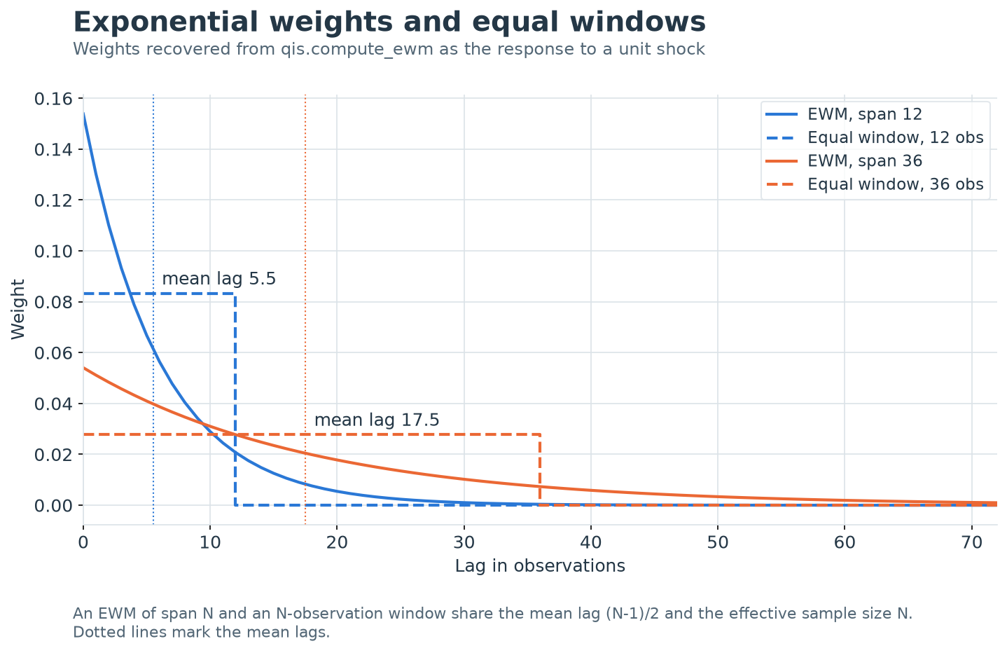
The exhibit recovers the weights \(\omega_k\) from qis.compute_ewm as the response to a unit shock and draws them against equal-weight windows of \(N=12\) and \(N=36\) observations. Each pair shares its mean lag, 5.5 and 17.5, and its effective sample size \(N\), as the identities above require. The EWM starts at \(2/(N+1)\), about twice the window weight, and decays geometrically with half-lives of 4.15 and 12.47 observations instead of stopping at lag \(N\).

Initial conditions

InitType selects the seed \(m_{-1}\) when no explicit init_value is passed. The seed is the state before a column’s first finite observation \(x_{t_0}\), which then updates it: \(m_{t_0}=\lambda m_{-1}+(1-\lambda)x_{t_0}\). It is computed on the scale of the series the recursion runs on, so in compute_ewm_vol it is a statistic of \(\tilde x^2\).

InitType	Seed \(m_{-1}\)	Information used
ZERO	0	None; \(x_{t_0}\) enters with weight \(1-\lambda\) and the output is shrunk towards zero by the factor \(1-\lambda^{t-t_0+1}\)
X0	The column’s first finite observation, so \(m_{t_0}=x_{t_0}\)	That observation only; pandas adjust=False
MEAN	Full-sample nanmean, 0 when a column is empty	The whole sample (look-ahead)
VAR	For a second-moment recursion, the full-sample variance of the observations with ddof=0	The whole sample (look-ahead)

By the unrolled recursion the seed keeps weight \(\lambda^{t-t_0+1}\) at row \(t\). It falls below 5% after \(\ln 20/(-\ln\lambda)\approx 1.5N\) rows: 54 rows at \(N=36\), 389 at \(N=260\). Until then a full-sample seed leaks later information into early estimates.

No default seeds with the full sample. Up to qis 5.30.3 compute_ewm_cross_xy seeded the denominators \(M^{xx}\) and \(M^{yy}\) of CrossXyType.BETA and CrossXyType.CORR with full-sample second moments (var_init_type=InitType.MEAN); it now seeds them with each column’s first square (InitType.X0), and var_init_type=InitType.MEAN restores the former seed. ewm_xy_convolution passes var_init_type=InitType.ZERO.

The other entry points of the chapter are point in time by default: compute_ewm, compute_ewm_vol, compute_ewm_newey_west_vol, compute_rolling_mean_adj, compute_ewm_beta_alpha_forecast, the optional mean adjustment of EwmLinearModel.fit and the vol-normalised covariance tensor use X0; compute_ewm_sharpe, compute_ewm_long_short_filter, compute_one_factor_ewm_betas, the moments of ewm_xy_convolution and the covariance functions start from zero. Before this release the vol-normalised tensor seeded its volatility with the full-sample mean of \(x^2\), EwmLinearModel.fit seeded its mean adjustment with full-sample means, and compute_ewm_beta_alpha_forecast defaulted to MEAN, which weighted its first beta towards the full-sample slope through the origin.

InitType.VAR seeds a second-moment recursion with the full-sample variance of the observations: in compute_ewm_vol and compute_ewm_newey_west_vol the seed is \(\operatorname{Var}(\tilde x)\), of order \(10^{-4}\) for daily returns with 1% volatility. A mean recursion cannot take it: compute_ewm and compute_rolling_mean_adj raise ValueError, and an EWMA mean adjustment requested together with VAR is seeded with MEAN. Before this release VAR seeded the variance with the variance of \(x^2\), of order \(10^{-8}\), and seeded a mean with a variance.

X0 takes each column’s first finite observation, so a column that starts after missing rows starts at \(m_{t_0}=x_{t_0}\), exactly like a column that starts on row 0, and its path is the one the same observations would give without the leading rows. Before its first observation a column’s output is missing. Before this release X0 took the first row, so a column that started late was seeded with 0 and started at \((1-\lambda)x_{t_0}\): with the leading missing row that qis.to_returns produces by default, the first EWM variance was \((1-\lambda)r_1^2\) and the first inverse-volatility weight \(1/\sqrt{1-\lambda}\approx 4.1\) times too large at \(\lambda=0.94\).

Mean adjustment

The volatility, Newey–West and cross-moment functions first replace \(x_t\) by \(\tilde x_t=x_t-\hat\mu_t\), with \(\hat\mu_t\) chosen by MeanAdjType:

MeanAdjType	\(\hat\mu_t\)	Timing and implementation notes
NONE	0	The second moment about zero, the default
INSAMPLE	Full-sample mean	Look-ahead. The nanmean of each column, repeated on every row, for DataFrames, Series and ndarrays
EXPANDING	Expanding mean of rows \(t_0,\dots,t\)	Point in time; includes \(x_t\), so \(\tilde x_{t_0}=0\)
EWMA	\(m_t\) with the same \(\lambda\)	Point in time; includes \(x_t\); seeded by init_type, so X0 gives \(\tilde x_{t_0}=0\)

For returns the difference between NONE and a centred estimate is usually small, because the squared mean is small relative to the variance. A 10% annual mean with 16% volatility adds \((0.1/252)^2\approx 1.6\times 10^{-7}\) to a daily variance of \(1.0\times 10^{-4}\), 0.16% of it; on a monthly grid the share is 3.3%. For signals, spreads and levels the difference is not small, and a second moment about zero is not a variance.

Identity (EWMA-centred residual). Because \(m_t\) includes \(x_t\),

\[ x_t-m_t=\lambda\,(x_t-m_{t-1}). \]

Proof. \(x_t-\lambda m_{t-1}-(1-\lambda)x_t=\lambda x_t-\lambda m_{t-1}\). \(\square\)

Proposition (shrinkage of EWMA-centred residuals). If \(x_t\) are IID with variance \(\sigma^2\), then in the stationary limit

\[ \mathbb{E}\big[(x_t-m_t)^2\big]=\frac{2\lambda^2}{1+\lambda}\,\sigma^2 =\frac{(N-1)^2}{N(N+1)}\,\sigma^2 . \]

Proof. \(x_t\) is independent of \(m_{t-1}\), \(\mathbb{E}m_{t-1}=\mathbb{E}x_t\), and \(\operatorname{Var}(m_{t-1})=\sigma^2(1-\lambda)/(1+\lambda)\) by the unit-variance proposition below. Hence \(\mathbb{E}(x_t-m_{t-1})^2=2\sigma^2/(1+\lambda)\); multiply by \(\lambda^2\) from the identity. \(\square\)

The factor is 0.920 at \(N=36\) and 0.989 at \(N=260\): an EWM volatility with MeanAdjType.EWMA is biased low by 4.1% and 0.6% respectively. It is the price of centring on a mean that has already seen the observation being centred.

Missing observations

NanBackfill decides the state at a row where the update is not finite, after a column’s first observation. The rule applies entry by entry, so in a covariance recursion a missing asset affects only its own row and column.

NanBackfill	State at a missing row	Output at the row
FFILL (default of the column-wise functions)	\(m_t=m_{t-1}\): time stops for this series	The state; pandas ignore_na=True
DEFLATED_FFILL (default of the covariance functions)	\(m_t=\lambda m_{t-1}\): the missing observation is a zero	The state
ZERO_FILL	\(m_t=0\): the memory is erased and the next observation gives \((1-\lambda)x_t\)	The state, 0
NAN_FILL	\(m_t=0\), as ZERO_FILL	Missing; an exact zero estimate elsewhere is reported as zero

Before a column’s first observation the output of the column-wise functions is missing under every policy. The matrix recursions have no per-column start: an asset that has not started holds the zero seed in its row and column, and NAN_FILL reports those entries as missing. Before this release ZERO_FILL and NAN_FILL returned zeros for leading missing rows, NAN_FILL returned no missing values outside the covariance tensors, and inside them it reported every entry that was exactly zero, a genuine zero covariance included, as missing.

Pitfall

A missing return that is economically a zero return corresponds to DEFLATED_FFILL, not to ZERO_FILL: ZERO_FILL sets the estimate to zero, so one missing daily return wipes out a year of variance history.

Volatility and annualisation

Definition. The EWM variance and volatility are

\[ v_t=\lambda v_{t-1}+(1-\lambda)\tilde x_t^2,\qquad \hat\sigma_t=\sqrt{\mathrm{AN}\,\max\big(v_t,\underline v_t\big)} . \]

compute_ewm_vol applies the steps in this order: mean adjustment, squaring, seeding (with X0, \(v_{t_0}=\tilde x_{t_0}^2\)), the recursion, the optional floor, warm-up masking, annualisation and the square root (apply_sqrt=False returns the variance). An explicit init_value is the seed \(v_{-1}\) before the first observation, so \(v_{t_0}=\lambda v_{-1}+(1-\lambda)\tilde x_{t_0}^2\).

• Annualisation. It applies when annualize=True or annualization_factor is given. For pandas input \(\mathrm{AN}\) is inferred from the index by qis.infer_annualisation_factor_from_df, which returns 12 for month-ends and 252 for business days, and falls back to 252 with a warning when no frequency can be inferred. A bare ndarray has no index and uses \(\mathrm{AN}=1\) with a warning. Otherwise \(\mathrm{AN}=1\).

• Floor. With vol_floor_quantile \(=\gamma\), \(\underline v_t\) is the trailing rolling \(\gamma\)-quantile of \(v\) over vol_floor_quantile_roll_period rows (default 1300, five years of 260 days), with at least 20% of the window present and the 'lower' interpolation. The floor is point in time. Since the square root is monotone, flooring the variance at its quantile is flooring the volatility at its quantile; \(\gamma=0.16\) is the suggested value. The floor works for DataFrames, Series and one- and two-dimensional ndarrays; before this release a Series raised ValueError and a one-dimensional ndarray returned a \(T\times T\) array.

• Warm-up. warmup_period sets that many leading finite values of each column to missing.

Covariance and correlation

Definition. For a vector of observations \(x_t\) of \(n\) assets, compute_ewm_covar and compute_ewm_covar_tensor run

\[ \hat\Sigma_t=\lambda\hat\Sigma_{t-1}+(1-\lambda)\,x_t x_t^{\top},\qquad t=0,\dots,T-1, \]

from the seed \(\hat\Sigma_{-1}\) given by covar0 (zero by default; non-finite entries become zero). The first returns \(\hat\Sigma_{T-1}\) and the second the whole path. Both the matrix and the scalar recursions update at row 0; the matrix recursions start from the zero seed and compute_ewm_vol from X0, so

\[ \operatorname{diag}\big(\hat\Sigma_t\big)=v_t-\lambda^{t+1}x_0^2 \]

elementwise, where \(v_t\) is the X0-seeded variance of compute_ewm_vol. The functions take \(x\) as given: there is no mean-adjustment argument, and a centred estimate requires demeaning the input first.

Proposition (positive semidefiniteness). If \(\hat\Sigma_{-1}\) is positive semidefinite and every \(x_t\) is complete, every \(\hat\Sigma_t\) is positive semidefinite.

Proof. For any vector \(a\), \(a^{\top}\hat\Sigma_t a=\lambda\,a^{\top}\hat\Sigma_{t-1}a+(1-\lambda)(a^{\top}x_t)^2\), which is non-negative if \(a^{\top}\hat\Sigma_{t-1}a\) is. Equivalently, \(\hat\Sigma_t\) is a combination with non-negative coefficients of the seed and of rank-one matrices \(x_s x_s^{\top}\). \(\square\)

The matrix is semidefinite, not definite: with a zero seed and fewer than \(n\) rows its rank is at most the number of rows.

Proposition (missing data). With missing entries, DEFLATED_FFILL, the default of the covariance functions, and ZERO_FILL (the state of NAN_FILL) preserve positive semidefiniteness; FFILL does not.

Proof. Under DEFLATED_FFILL the row and column of a missing asset \(i\) become \(\lambda\hat\Sigma_{t-1}\), which is exactly the full update with \(x_{i,t}\) replaced by zero; apply the previous proposition. Under ZERO_FILL the block of observed assets is updated with their observed sub-vector, a principal submatrix of a semidefinite matrix plus a rank-one term, and the rest is set to zero; padding a semidefinite block with zero rows and columns keeps it semidefinite. For FFILL, take \(\lambda=0.94\), the seed with unit diagonal and off-diagonal 0.99, and \(x_t=(\text{missing},0)\): the held entries give \(\begin{pmatrix}1&0.99\\0.99&0.94\end{pmatrix}\), whose determinant \(0.94-0.99^2=-0.0401\) is negative. \(\square\)

Pitfall

Asynchronous gaps, such as exchange holidays in a multi-country panel, combined with an explicit NanBackfill.FFILL can produce EWM covariance matrices with negative eigenvalues and correlations above one. compute_ewm_covar, compute_ewm_covar_tensor, compute_ewm_covar_tensor_vol_norm_returns and compute_ewm_covar_newey_west therefore default to DEFLATED_FFILL, which is also the default path of compute_ewm_corr_df and compute_data_pca_r2; before this release they defaulted to FFILL.

With is_corr=True each matrix is converted to a correlation matrix \(\hat\Sigma_{ij}/\sqrt{\hat\Sigma_{ii}\hat\Sigma_{jj}}\) (entries of assets without positive variance are missing, the diagonal is one). An EWM correlation of raw returns is uncentred: it is the weighted cosine of two return vectors, not the Pearson correlation, unless the returns are mean-adjusted first. For one-dimensional input compute_ewm_covar makes a single update and, like the two-dimensional path, honours is_corr.

Vol-normalised covariance. compute_ewm_covar_tensor_vol_norm_returns estimates the correlation on returns scaled by their own EWM volatility and rescales it:

\[\begin{split} \begin{aligned} v_t&=\lambda v_{t-1}+(1-\lambda)x_t^2,\qquad v_{-1}=x_{t_0}^2,\\ \Gamma_t&=\lambda\Gamma_{t-1}+(1-\lambda)\,z_t z_t^{\top},\qquad z_{i,t}=x_{i,t}/\hat\sigma_{i,t},\\ \hat\Sigma_t&=\operatorname{diag}(\hat\sigma_t)\,\hat\rho_t\,\operatorname{diag}(\hat\sigma_t), \qquad \hat\rho_t=\text{the correlation matrix of }\Gamma_t , \end{aligned} \end{split}\]

elementwise in \(i\) for the first line, with \(\hat\sigma_{i,t}=\sqrt{v_{i,t}}\), the seed \(v_{-1}\) the column’s first finite squared return (X0, so the first volatility of a column is the absolute value of its first return) and \(\Gamma_{-1}\) given by covar0. The function returns \((\hat\Sigma_t,\Gamma_t,\hat\sigma_t)\) as tensors of shape \((T,n,n)\), \((T,n,n)\) and \((T,n)\); with is_corr=True the second output is \(\hat\rho_t\) and the first is unchanged. Every output is point in time; before this release the volatility seed was the full-sample mean of \(x^2\). Scaling first prevents a volatile episode or asset from dominating the correlation estimate. It also caps the normalised returns: at every row \(v_t\ge(1-\lambda)x_t^2\), so

\[ \lvert z_{i,t}\rvert\le\frac{1}{\sqrt{1-\lambda}}=\sqrt{\frac{N+1}{2}}, \]

4.30 at \(N=36\). Every \(\hat\Sigma_t\) is positive semidefinite, being a congruence of the correlation matrix of a semidefinite matrix.

Betas and cross moments

compute_ewm_cross_xy forms the products after the optional mean adjustment (seeded by init_type), then runs three recursions:

\[ M^{xy}_t=\lambda M^{xy}_{t-1}+(1-\lambda)\tilde x_t\tilde y_t,\qquad M^{xx}_t=\lambda M^{xx}_{t-1}+(1-\lambda)\tilde x_t^2,\qquad M^{yy}_t=\lambda M^{yy}_{t-1}+(1-\lambda)\tilde y_t^2 . \]

\(M^{xy}\) is seeded by init_type (default ZERO, so the first product enters with weight \(1-\lambda\)) and \(M^{xx}\), \(M^{yy}\) by var_init_type (default X0, the first squares). The first beta is therefore \((1-\lambda)\,y_1/x_1\), shrunk towards zero while \(M^{xy}\) warms up; var_init_type=InitType.ZERO gives the raw ratio \(y_1/x_1\) instead, which is unstable over the first rows. warmup_period \(=k\) masks an output until its pair has \(k+1\) joint observations, counted from the pair’s own first one. Up to qis 5.30.3 the default MEAN seeded the denominators with full-sample second moments, a look-ahead that damped the ratios over the first \(1.5N\) rows.

CrossXyType	Output	Notes
COVAR (default)	\(M^{xy}_t\)	A cross moment about zero unless mean-adjusted
BETA	\(\hat\beta_t=M^{xy}_t/M^{xx}_t\)	Missing where \(M^{xx}_t\) is not positive
CORR	\(\hat\rho_t=M^{xy}_t/\sqrt{M^{xx}_tM^{yy}_t}\)	Uncentred unless mean-adjusted; missing where the denominator is not positive

Both tests are scale free. Before this release they masked any denominator below \(10^{-8}\), which silenced a factor with a daily volatility of one basis point.

On complete data and with the default seeds, \(\lvert\hat\rho_t\rvert\le 1\) by the Cauchy–Schwarz inequality, because the numerator’s seed is zero and the denominators’ seeds are non-negative. The function pairs two DataFrames of equal shape column by column, a Series factor with every column of a DataFrame or with a Series (after an inner join of the indices), and two ndarrays of the same shape, one- or two-dimensional; a DataFrame factor with a Series asset raises TypeError.

compute_one_factor_ewm_betas(x, y) is the one-factor beta for a Series factor and a DataFrame of assets on an identical index. It has no mean adjustment and zero seeds, updates at row 0, and applies nan_backfill to both moments:

\[ \hat\beta_{j,t}=\frac{M^{x y_j}_t}{M^{xx}_t},\qquad M^{xy}_{-1}=M^{xx}_{-1}=0 . \]

The rows \(t\le\) warmup_period (20 by default, so 21 rows) are missing to suppress the unstable start, and the beta is missing where \(M^{xx}_t\) is not positive. The multi-factor kernel qis.compute_ewm_xy_beta_tensor solves \(\hat B_t=(M^{xx}_t)^{-1}M^{xy}_t\) with a scale-free test: a factor whose second moment is not positive gets missing betas and the others are solved from the reduced system, and when the reduced matrix, rescaled to unit diagonal, has its smallest eigenvalue below \(10^{-12}\) times its largest, every beta is missing. Before this release a factor second moment below \(10^{-8}\), in the units of \(x^2\), replaced the inverse by the identity for every factor and reported the raw cross moment as the beta.

compute_ewm_beta_alpha_forecast(x_data, y_data, span) adds an intercept and a forecast to the one-factor beta. With seeds X0 by default, it returns \(\hat\beta_t=M^{xy}_t/M^{xx}_t\), the alpha \(\hat\alpha_t\) as the EWM of the fitted residual \(y_t-\hat\beta_t x_t\), the one-step-ahead prediction \(\hat\beta_{t-1}x_t+\hat\alpha_{t-1}\), which is missing on the first row, and in-sample residual variance and \(R^2\) of \(y_t-\hat\beta_t x_t-\hat\alpha_t\). A prior beta_init_value \(=\beta_0\) replaces the first informative pair \((x_f,y_f)\) by \((x_f,\beta_0x_f)\) and seeds both moments with it, so the first beta is \(\beta_0\) and the prior keeps weight \(\lambda^{t-f}\). Before this release the default seed was MEAN, the prediction used \(\hat\beta_t\) and \(\hat\alpha_t\), and the beta moments ignored nan_backfill.

ewm_xy_convolution(returns, freq, signals, convolution_type) measures lagged dependence at a horizon of \(h\) rows, \(h\) being get_annualization_factor(freq) as a whole number: 252 for 'B', 52 for 'W-WED', 12 for 'ME', 4 for 'QE'. Every frequency with a whole-number factor runs; one without raises ValueError. The input is assumed daily, so freq='ME' means 12 rows, not one month. The decay is \(\lambda=1-2/(h+1)\) (0.2 when \(h=1\)). Returns are optionally divided by their compute_ewm_vol volatility at decay 0.94 lagged one row (is_ra_returns=True) and summed over \(h\) rows, \(R_t=\sum_{j=0}^{h-1}r_{t-j}\). ConvolutionType.AUTO_CORR correlates \(R_{t-h}\) with \(R_t\); SIGNAL_CORR and SIGNAL_BETA correlate or regress \(R_t\) on the signal (its last value or its \(h\)-row mean) shifted by \(h\) rows. The call is compute_ewm_cross_xy with the zero seed of the cross moment and var_init_type=InitType.ZERO for the denominators, so every estimate is point in time; before this release the denominators carried the full-sample MEAN seed that was then the default of compute_ewm_cross_xy. Overlapping \(h\)-row sums make consecutive products strongly dependent; see serial dependence and signal diagnostics.

Unit-variance scaling

Proposition (variance of an EWM of white noise). If \(\xi_t\) are IID with mean zero and unit variance and the seed is zero, then

\[\begin{split} \begin{aligned} \operatorname{Var}(m_t)=\operatorname{Var}\Big(\sum_{k=0}^{t}(1-\lambda)\lambda^k\xi_{t-k}\Big) &=\frac{1-\lambda}{1+\lambda}\big(1-\lambda^{2t+2}\big)\\ &\longrightarrow\ \frac{1-\lambda}{1+\lambda}=\frac{1}{N}. \end{aligned} \end{split}\]

Proof. Independence makes the variance the sum of squared weights, \((1-\lambda)^2\sum_{k\le t}\lambda^{2k}=(1-\lambda)^2(1-\lambda^{2t+2})/(1-\lambda^2)\); cancel \(1-\lambda\). \(\square\)

The stationary variance \(1/N\) is that of an \(N\)-observation equal-weight mean, which restates \(N_{\mathrm{eff}}=N\). Multiplying by \(\sqrt{(1+\lambda)/(1-\lambda)}=\sqrt{N}\) therefore gives unit variance; this is is_unit_vol_scaling=True in ewm_recursion and compute_ewm. With a non-zero seed the variance approaches the same limit.

compute_ewm_std1_norm(data, span=260) builds a unit-variance smoothed signal in three steps: \(\tilde x_t=x_t-m_t\) with the same-span EWMA mean (is_demean=True, MeanAdjType.EWMA), a volatility \(\hat\sigma_t\) from the X0-seeded EWM of \(\tilde x^2\), and the output \(\eta\sqrt{N}\,\mathcal{E}_\lambda(\tilde x/\hat\sigma)_t\), the last EWM seeded at zero, with \(\eta=\sqrt{1+\lambda}\) under the same-span EWMA demeaning and \(\eta=1\) otherwise, and missing values set to zero by default. The ratio is missing where \(\hat\sigma_t\) is below \(10^{-8}\); because \(v_t\ge(1-\lambda)\tilde x_t^2\) it is bounded by \(1/\sqrt{1-\lambda}\), and it equals that bound (11.4 at \(N=260\)) at the first update after \(\tilde x_{t_0}=0\), a warm-up transient.

Proposition (variance of the demeaned signal). Let \(x_t\) be IID with variance \(\sigma^2\) and replace \(\hat\sigma_t\) by its stationary level. Then \(\sqrt{N}\,\mathcal{E}_\lambda(\tilde x/\hat\sigma)_t\) with \(\tilde x=x-\mathcal{E}_\lambda(x)\) has stationary variance \(1/(1+\lambda)\), so \(\eta=\sqrt{1+\lambda}\) restores unit variance.

Proof. The map \(x\mapsto\mathcal{E}_\lambda\big(x-\mathcal{E}_\lambda(x)\big)\) has weights \(h_k-(h*h)_k=(1-\lambda)\lambda^k\big(1-(1-\lambda)(k+1)\big)\), with \(h_k=(1-\lambda)\lambda^k\); summing three geometric series, their squares add up to \(2\lambda^2(1-\lambda)/(1+\lambda)^3\). By the shrinkage proposition \(\hat\sigma^2=\mathbb{E}\tilde x_t^2=2\lambda^2\sigma^2/(1+\lambda)\). Hence the variance is \(N\cdot 2\lambda^2(1-\lambda)(1+\lambda)^{-3}\big/\big(2\lambda^2/(1+\lambda) \big)=N(1-\lambda)/(1+\lambda)^2=1/(1+\lambda)\). \(\square\)

The squared weights of the linear map scaled by \(\sqrt{N}\) sum to \(2\lambda^2/(1+\lambda)^2\), 0.496 at \(N=260\), and the output standard deviation without \(\eta\) is \(1/\sqrt{1+\lambda}=0.71\). Before this release compute_ewm_std1_norm returned that 0.71, although its docstring promised unit standard deviation, and seeded the last EWM with its first value, a transient of up to \(\sqrt{N}\) standard deviations.

The two-span long–short filter

compute_ewm_long_short_filter(data, long_span=63, short_span=5) combines two EWMs seeded at zero before the first observation, which enters with weight \(1-\lambda\); a missing row holds both legs (FFILL). In the code each leg is weight * load * EWM, with load \(\sqrt{(1+\lambda)/(1-\lambda)}\) and weight \(1/\big(\sqrt{1-\lambda^2}\,\kappa\big)\). Their product is \(1/\big((1-\lambda)\kappa\big)\), which turns each leg into the unnormalised sum \(\kappa^{-1}\sum_k\lambda^k x_{t-k}\):

\[ F_t=\frac{1}{\kappa}\sum_{k=0}^{t}\big(\lambda_L^k-\lambda_S^k\big)\,x_{t-k},\qquad \kappa^2=\frac{1}{1-\lambda_L^2}+\frac{1}{1-\lambda_S^2}-\frac{2}{1-\lambda_L\lambda_S}. \]

Proposition (unit variance). For IID unit-variance input the stationary variance of \(F_t\) is one.

Proof. The variance is \(\kappa^{-2}\sum_{k\ge 0}(\lambda_L^k-\lambda_S^k)^2\). Expanding the square gives three geometric series, \(\sum\lambda_L^{2k}=1/(1-\lambda_L^2)\), \(\sum\lambda_S^{2k}=1/(1-\lambda_S^2)\) and \(\sum(\lambda_L\lambda_S)^k=1/(1-\lambda_L\lambda_S)\), whose combination is \(\kappa^2\). \(\square\)

With short_span=None the filter is \(\sqrt{(1+\lambda_L)/(1-\lambda_L)}\,m_t\), unit variance by the previous proposition. With two legs the weight at lag 0 is \(\lambda_L^0-\lambda_S^0=0\): \(F_t\) does not depend on \(x_t\) and is known one row earlier.

Identity (moving-average crossover). Let \(X_t=\sum_{j=0}^{t}x_j\) with \(X_{-1}=0\) and let \(\mathcal{E}_\lambda(X)\) be the EWM of \(X\) seeded at zero, the state \(X_{-1}\) before row 0. Then for \(t\ge 0\)

\[ \kappa\,F_{t+1}=\mathcal{E}_{\lambda_S}(X)_t-\mathcal{E}_{\lambda_L}(X)_t . \]

Proof. By the unrolled recursion with a zero seed and \(X_t-X_{t-k}=\sum_{j<k}x_{t-j}\), \(X_t-\mathcal{E}_\lambda(X)_t=\lambda^{t+1}X_t+\sum_{k=1}^{t}(1-\lambda)\lambda^k(X_t-X_{t-k}) =\sum_{j=0}^{t}\lambda^{j+1}x_{t-j}\). Subtract this for \(\lambda_S\) from the same for \(\lambda_L\), and compare with \(\kappa F_{t+1}=\sum_{k=1}^{t+1}(\lambda_L^k-\lambda_S^k)x_{t+1-k}\). \(\square\)

With log returns \(X_t\) is the log price relative, so the filter is the fast-minus-slow EWMA crossover of log prices, lagged one row and scaled to unit variance under white noise. The kernel is hump-shaped with its maximum at lag \(\ln(\ln\lambda_S/\ln\lambda_L)/\ln(\lambda_L/\lambda_S)\), 6.8 rows for the defaults, and its response to a permanent unit shift in \(x\) is \(\sum_k(\lambda_L^k-\lambda_S^k)/\kappa=(N_L-N_S)/(2\kappa)\), 8.23 for the defaults (\(\kappa=3.52\)). Signals of this type are smoothed versions of the time-series momentum of Moskowitz, Ooi and Pedersen (2012), which trades on the sign of the past twelve-month return.

The spans are validated: both must be at least 1 (span 1 is a pass-through with \(\lambda=0\)), and short_span must be strictly below long_span, since equal spans give \(\kappa=0\). The first warmup_period=21 finite values are set to missing. The filter takes DataFrames, Series and one- or two-dimensional ndarrays; the numba kernel compute_ewm_long_short does no validation. Before this release a finite first row was dropped from both legs, and a one-dimensional ndarray failed in numba.

Newey–West EWM variance

Definition. compute_ewm_newey_west_vol(data, num_lags=q) corrects the EWM variance of compute_ewm_vol with Bartlett-weighted EWM autocovariances of the mean-adjusted series:

\[\begin{split} \begin{aligned} v^{\mathrm{NW}}_t&=v_t+\sum_{k=1}^{q}\Big(1-\frac{k}{q+1}\Big)\,2\,\lambda^{k/2}c_{k,t},\\ c_{k,t}&=\lambda c_{k,t-1}+(1-\lambda)\,\tilde x_t\tilde x_{t-k}\ \ (t\ge k), \qquad c_{k,t}=0\ \ (t<k). \end{aligned} \end{split}\]

\(v_t\) is seeded with \(\tilde x_{t_0}^2\) under X0, as in compute_ewm_vol, so num_lags=0 reproduces the EWM variance exactly; every lag term uses the same decay (given by span or ewm_lambda). In \(c_{k,t}\) the product \(\tilde x_s\tilde x_{s-k}\) carries the weight \((1-\lambda)\lambda^{t-s}\) of its later date; the factor \(\lambda^{k/2}\) turns it into \((1-\lambda)\lambda^{t-s+k/2}\), the geometric mean of the weights of its two dates. The Bartlett weights are those of Newey and West (1987); the regression use of the same kernel is in regression and HAC inference.

Proposition (non-negativity). For a seed \(v_{-1}\ge 0\), \(v^{\mathrm{NW}}_t\ge 0\) at every row.

Proof. Put \(g_s=\sqrt{(1-\lambda)\lambda^{t-s}}\,\tilde x_s\) for \(t_0\le s\le t\) and \(g_s=0\) otherwise. With the geometric-mean weights, \(v^{\mathrm{NW}}_t=\lambda^{t-t_0+1}v_{-1}+\sum_{s,s'}g_sg_{s'}K(s-s')\). The number of integers \(j\) with both \(j-s\) and \(j-s'\) in \(\{0,\dots,q\}\) is \((q+1)K(s-s')\), so \(\sum_{s,s'}g_sg_{s'}K(s-s')=(q+1)^{-1}\sum_j\big(\sum_{i=0}^{q}g_{j-i}\big)^2\ge 0\). \(\square\)

The same argument covers the missing-data policies, each of which is the quadratic form of a modified sequence: FFILL holds the estimate at a gap and pairs each observation with the previous observed ones, the estimator on the observed rows; DEFLATED_FFILL makes the gap a zero observation; ZERO_FILL and NAN_FILL restart the estimator after the gap, NAN_FILL reporting the gap as missing. The second output is the ratio \(v^{\mathrm{NW}}_t/v_t\), missing where \(v_t\) is not positive. Annualisation multiplies \(v^{\mathrm{NW}}_t\) by \(\mathrm{AN}\), and the square root is taken last. compute_ewm_covar_newey_west is the matrix analogue, with the same factor \(\lambda^{k/2}\), and is positive semidefinite for complete data and DEFLATED_FFILL gaps by the same argument applied to \(a^{\top}x_s\).

For \(x_t=(-1)^t\lambda^{t/2}\), \(q=1\) and the X0 seed, \(v_t=\lambda^t\big(1+(1-\lambda)t\big)\) and \(c_{1,t}=-(1-\lambda)\,t\,\lambda^{t-1/2}\), so \(v^{\mathrm{NW}}_t=\lambda^t\): the quadratic form contributes \((1-\lambda)\lambda^t\) and the seed \(\lambda^{t+1}\). Without the factor \(\lambda^{1/2}\), as before this release, the estimator was \(\lambda^t\big(1-(1-\lambda)t(\lambda^{-1/2}-1)\big)\), negative from row 531 at \(\lambda=0.94\), and qis reported a missing volatility; the lag recursions also ignored nan_backfill and, in the matrix version, ewm_lambda. The factor shrinks the lag-\(k\) term by 3% per lag at \(\lambda=0.94\) relative to that estimator.

EWM Sharpe ratios

compute_ewm_sharpe(returns, span=260, norm_type=1) fills missing returns with zero, infers \(\mathrm{AN}\) from the index and runs \(m_t\) and a second-moment recursion from zero seeds, the states before row 0, so the first return enters with weight \(1-\lambda\) (before this release it was discarded). With initial_sharpes \(=\mathrm{SR}_0\) the seeds are instead a prior with 10% annual volatility, \(m_{-1}=0.1\,\mathrm{SR}_0/\mathrm{AN}\) and \(v_{-1}=0.01/\mathrm{AN}\).

norm_type	Output \(\mathrm{SR}^{(n)}_t\)	Reading
0	\(\mathrm{AN}\,m_t\)	Annualised EWM mean return, not a ratio
1 (default)	\(\sqrt{\mathrm{AN}}\,m_t\big/\sqrt{\mathcal{E}_\lambda(x^2)_t}\)	Mean over root mean square
2	\(\sqrt{\mathrm{AN}}\,m_t\big/\sqrt{\mathcal{E}_\lambda\big((x-m)^2\big)_t}\)	Mean over the root EWM of squared deviations from the running mean \(m_s\)

Norms 1 and 2 are missing where the denominator is zero, which happens only while every return so far is zero. Norm 1 divides by the root mean square, the second moment about zero of the MeanAdjType.NONE convention; norm 2 divides by the EWM deviation from the running mean.

Proposition (EWM Sharpe biases). With zero seeds, \(\lvert\mathrm{SR}^{(1)}_t\rvert\le\sqrt{\mathrm{AN}}\). For IID returns with per-period Sharpe ratio \(s=\mu/\sigma\), the ratio of stationary expectations is \(\sqrt{\mathrm{AN}}\,s/\sqrt{1+s^2}\) for norm 1 and \(\sqrt{\mathrm{AN}}\,s\,\sqrt{N(N+1)}/(N-1)\) for norm 2.

Proof. The weights of \(m_t\) sum to \(1-\lambda^{t+1}\le 1\), so by Cauchy–Schwarz \(m_t^2\le\mathcal{E}_\lambda(x^2)_t\). The stationary expectations are \(\mathbb{E}m_t=\mu\) and \(\mathbb{E}x^2=\mu^2+\sigma^2\), which gives norm 1; for norm 2 use the shrinkage proposition, \(\mathbb{E}(x_t-m_t)^2=\sigma^2(N-1)^2/(N(N+1))\). \(\square\)

Norm 1 compresses the annualised Sharpe ratio \(\mathrm{SR}\) by the factor \(1/\sqrt{1+\mathrm{SR}^2/\mathrm{AN}}\): by 4% for \(\mathrm{SR}=1\) on monthly data and by 0.2% on daily data. Norm 2 inflates it by 4.3% at \(N=36\) and 0.6% at \(N=260\). Both statements are about ratios of expectations; the ratio of two noisy EWMs has additional small-sample bias. compute_ewm_sharpe_from_prices resamples prices to freq (default 'QE'), takes log returns and calls norm 2 with span 40.

EWM score and outlier filtering

Definition. compute_ewm_score(data, ewm_lambda=0.94) returns \((m_t,z_t)\) with

\[ z_t=\frac{x_t-m_t}{\max(\hat\sigma_t,\,c)}, \]

where \(m_t\) is the X0-seeded EWM mean, \(\hat\sigma_t\) the compute_ewm_vol volatility about zero and \(c\) the full-sample clip_quantile (0.16) quantile of the column’s own \(\hat\sigma\) (is_clip=True; before this release the quantile was pooled over all columns). The score is missing where \(x_t\) is. Both \(m_t\) and \(\hat\sigma_t\) include \(x_t\), and \(c\) uses the whole sample.

Proposition (score bound). At every row with \(x_t\) observed,

\[ \lvert z_t\rvert\le\sqrt{\frac{\lambda}{1-\lambda}}=\sqrt{\frac{N-1}{2}}, \]

3.96 at \(\lambda=0.94\), and the bound is sharp.

Proof. \(m_t\) and \(v_t\) are the mean and second moment of one discrete distribution: the seed \(x_{t_0}\) and the observations, with the same weights, of which \(x_t\) has weight \(p=1-\lambda\). Write \(m_t=p\,x_t+(1-p)\mu'\), with \(\mu'\) the mean of the other mass. The variance of the distribution is at least its between-group part, \(p(x_t-m_t)^2+(1-p)(\mu'-m_t)^2=p(x_t-m_t)^2/(1-p)\). Hence \((x_t-m_t)^2\le\frac{1-p}{p}(v_t-m_t^2)\le\frac{\lambda}{1-\lambda}v_t\); clipping only raises the denominator. Equality holds when the other mass sits at one point \(\mu'\) and \(m_t=0\). \(\square\)

Insight

Because the score is measured against estimates that already contain the observation, a single observation can never score above \(\sqrt{(N-1)/2}\), however extreme. A threshold can bind only if \(\lambda>c^2/(1+c^2)\) for a cut at \(c\): \(\lambda>0.990\) for \(c=10\). From a zero-mean state a move of \(k\) standard deviations scores \(\lambda k/\sqrt{\lambda+(1-\lambda)k^2}\), which rises to \(\lambda/\sqrt{1-\lambda}=3.84\) at \(\lambda=0.94\): 3.01 for \(k=5\) and 3.57 for \(k=10\).

The preset policies SOFT_RANGE_CEIL_POLICY and SOFT_POSITIVE_LOG_POLICY of the internal enum qis.models.linear.ewm_winsor_outliers.OutlierPolicyTypes cut the score at 3.57, the score of a 10-standard-deviation move, computed by the internal helper score_of_move. Before this release they cut at 10, which the score can never reach at \(\lambda=0.94\).

filter_outliers(data, outlier_policy) applies a qis.OutlierPolicy in this order, setting rejected points to missing: the absolute ceiling and floor; the optional log transform (which requires abs_floor); a cut at the full-sample nanmean plus std_abs_ceil (or std_abs_floor) times the full-sample nanstd with ddof=0; a cut of the EWM score of the cleaned data at std_ewm_ceil and std_ewm_floor; and the inverse log. With nan_replacement_type=ReplacementType.EWMA_MEAN every non-finite value, including the input’s own missing values, is then replaced by the EWM mean of the cleaned data; otherwise rejected and missing points stay missing. Invalid-value warnings are silenced for the duration of the call only (before this release the call changed numpy’s error state for the rest of the process).

ewm_insample_winsorising(data, ewm_lambda=0.94, quantile_cut=0.025) computes \(z_t\), then the full-sample quantile_cut and 1 - quantile_cut quantiles of \(z\) per column. Points outside are replaced by \(m_t\) (EWMA_MEAN, the default), set missing (NAN), or, for QUANTILES, replaced by the corresponding full-sample quantile of the data, not of the score. The quantiles ignore missing values, so a column with gaps is winsorised like any other (before this release one missing value left the whole column unchanged). All three functions use the full sample and belong in descriptive cleaning, not in a backtest. The non-anticipating variant, the internal qis.models.linear.ewm_winsor_outliers.ewm_winsdor_markovian_score, scores \(x_t\) against the state at \(t-1\) and leaves the state unchanged at an outlier or a missing value, for one series or a panel alike.

Worked example

The first block runs the recursion by hand on three numbers with \(\lambda=0.5\), the decay of span 3. With the X0 seed the outputs are 2, then \(0.5\cdot 2+0.5\cdot 4=3\), then \(0.5\cdot 3+0.5\cdot 0=1.5\), which pandas reproduces with adjust=False. With the ZERO seed the first number enters with weight one half: 1, 2.5, 1.25. The same numbers after two missing rows give the same path, two rows later. On a series with two interior missing rows the four NanBackfill policies give the values in the table of the missing-data section: FFILL equals pandas with ignore_na=True, DEFLATED_FFILL equals the recursion with the gaps filled by zeros, and before the first observation every policy returns missing values.

import numpy as np
import pandas as pd
import qis

x = pd.Series([2.0, 4.0, 0.0])
m_x0 = qis.compute_ewm(x, ewm_lambda=0.5)
np.testing.assert_allclose(m_x0, [2.0, 3.0, 1.5])
np.testing.assert_allclose(qis.compute_ewm(x, span=3), m_x0)
np.testing.assert_allclose(x.ewm(span=3, adjust=False).mean(), m_x0)
np.testing.assert_allclose(qis.compute_ewm(x, ewm_lambda=0.5, init_type=qis.InitType.ZERO),
                           [1.0, 2.5, 1.25])
late = pd.Series([np.nan, np.nan, 2.0, 4.0, 0.0])
np.testing.assert_allclose(qis.compute_ewm(late, ewm_lambda=0.5), [np.nan, np.nan, 2.0, 3.0, 1.5])

gappy = pd.Series([1.0, 2.0, np.nan, np.nan, 4.0])
expected = {qis.NanBackfill.FFILL: [1.0, 1.5, 1.5, 1.5, 2.75],
            qis.NanBackfill.DEFLATED_FFILL: [1.0, 1.5, 0.75, 0.375, 2.1875],
            qis.NanBackfill.ZERO_FILL: [1.0, 1.5, 0.0, 0.0, 2.0],
            qis.NanBackfill.NAN_FILL: [1.0, 1.5, np.nan, np.nan, 2.0]}
for policy, values in expected.items():
    np.testing.assert_allclose(qis.compute_ewm(gappy, ewm_lambda=0.5, nan_backfill=policy), values)
    leading = qis.compute_ewm(pd.concat([pd.Series([np.nan]), gappy], ignore_index=True),
                              ewm_lambda=0.5, nan_backfill=policy)
    np.testing.assert_allclose(leading, [np.nan] + values)
np.testing.assert_allclose(qis.compute_ewm(gappy.fillna(0.0), ewm_lambda=0.5),
                           expected[qis.NanBackfill.DEFLATED_FFILL])
np.testing.assert_allclose(gappy.ewm(alpha=0.5, adjust=False, ignore_na=True).mean(),
                           expected[qis.NanBackfill.FFILL])

The second block checks the span table against the weights themselves: the mean lag and the Kish size are computed by summing the weight series, and the half-life is checked by counting how many lags hold half the weight.

lags = np.arange(20_000)
rows = []
for span in [12, 36, 52, 260]:
    decay = 1.0 - 2.0 / (span + 1.0)
    omega = (1.0 - decay) * decay ** lags
    mean_lag = np.sum(lags * omega)
    n_eff = omega.sum() ** 2 / np.sum(omega ** 2)
    half_life = np.log(2.0) / -np.log(decay)
    assert np.isclose(mean_lag, (span - 1) / 2) and np.isclose(n_eff, span)
    assert omega[:int(half_life)].sum() < 0.5 < omega[:int(half_life) + 1].sum()
    tail_lag = np.log(20.0) / -np.log(decay)
    assert np.isclose(omega[lags >= tail_lag].sum(), 0.05, atol=(1 - decay) * 0.05)
    rows.append([decay, half_life, mean_lag, n_eff, tail_lag])
table = pd.DataFrame(rows, index=[12, 36, 52, 260],
                     columns=['lambda', 'half-life', 'mean lag', 'effective N', '5% tail lag'])
np.testing.assert_allclose(table['lambda'], [0.8462, 0.9459, 0.9623, 0.9923], atol=5e-5)
np.testing.assert_allclose(table['half-life'], [4.15, 12.47, 18.02, 90.11], atol=5e-3)
np.testing.assert_allclose(table['5% tail lag'], [17.9, 53.9, 77.9, 389.4], atol=0.05)
np.testing.assert_allclose(table['half-life'], np.log(2.0) / 2 * table.index, atol=0.12 / 12)

The third block uses 119 month-end simple returns (February 2015 to December 2024) of the synthetic US equity and Treasury series. compute_ewm with span 36 equals pandas ewm(span=36, adjust=False), and the annualised compute_ewm_vol equals \(\sqrt{12\,v_t}\) from an independent loop seeded with \(x_0^2\). The index is month-end, so qis infers \(\mathrm{AN}=12\). The last EWM volatilities are 19.3% for equities and 5.9% for Treasuries, against full-sample volatilities of 18.5% and 5.8%. With the leading missing row that qis.to_returns keeps by default, the first volatility is the absolute first return, and the rest of the path is unchanged. InitType.VAR seeds the variance with the sample variance of the returns, and compute_ewm rejects it.

from qis.datasets import generate_synthetic_universe

universe = generate_synthetic_universe(start='2015-01-01', end='2024-12-31', seed=20260725,
                                       apply_quirks=False)
prices = universe.prices[['SEQ_US', 'SBD_TSY']].resample('ME').last()
returns = qis.to_returns(prices, is_log_returns=False, drop_first=True)
span = 36
lam = 1.0 - 2.0 / (span + 1.0)
assert len(returns) == 119 and qis.infer_annualisation_factor_from_df(returns) == 12.0

np.testing.assert_allclose(qis.compute_ewm(returns, span=span),
                           returns.ewm(span=span, adjust=False).mean(), atol=1e-15)

r = returns.to_numpy()
v = np.empty_like(r)
v[0] = r[0] ** 2
for t in range(1, len(r)):
    v[t] = lam * v[t - 1] + (1.0 - lam) * r[t] ** 2
vol = qis.compute_ewm_vol(returns, span=span, annualize=True)
np.testing.assert_allclose(vol, np.sqrt(12.0 * v), rtol=1e-12)
np.testing.assert_allclose(vol.iloc[-1], [0.193, 0.059], atol=5e-4)
np.testing.assert_allclose(returns.std() * np.sqrt(12.0), [0.185, 0.058], atol=5e-4)

with_leading_row = qis.to_returns(prices, is_log_returns=False)
assert with_leading_row.iloc[0].isna().all()
vol_leading = qis.compute_ewm_vol(with_leading_row, span=span, annualize=True)
np.testing.assert_allclose(vol_leading.iloc[1:], vol, rtol=1e-12)
np.testing.assert_allclose(vol_leading.iloc[1], np.sqrt(12.0) * np.abs(r[0]), rtol=1e-12)

var_seeded = qis.compute_ewm_vol(returns, span=span, init_type=qis.InitType.VAR, apply_sqrt=False)
np.testing.assert_allclose(var_seeded.iloc[0], lam * r.var(axis=0) + (1.0 - lam) * r[0] ** 2)
try:
    qis.compute_ewm(returns, init_type=qis.InitType.VAR)
    raise AssertionError('a mean cannot take a variance seed')
except ValueError:
    pass

The fourth block checks the covariance results. On complete data the final matrix is semidefinite and its diagonal differs from the X0 variance by \(\lambda^{T}x_0^2\). With the counterexample of the proof and an explicit FFILL, the smallest eigenvalue is −0.020; the default DEFLATED_FFILL returns \(0.94\) times the seed, which is positive definite. A one-dimensional input with is_corr=True returns a correlation matrix.

cov = qis.compute_ewm_covar(r, span=span)
assert np.linalg.eigvalsh(cov).min() >= 0.0
np.testing.assert_allclose(np.diag(cov), v[-1] - lam ** len(r) * r[0] ** 2, rtol=1e-10)

seed = np.array([[1.0, 0.99], [0.99, 1.0]])
one_gap = np.array([[np.nan, 0.0]])
held = qis.compute_ewm_covar(one_gap, ewm_lambda=0.94, covar0=seed,
                             nan_backfill=qis.NanBackfill.FFILL)
np.testing.assert_allclose(held, [[1.0, 0.99], [0.99, 0.94]])
np.testing.assert_allclose(np.linalg.eigvalsh(held).min(), -0.0205, atol=5e-5)
deflated = qis.compute_ewm_covar(one_gap, ewm_lambda=0.94, covar0=seed)
np.testing.assert_allclose(deflated, 0.94 * seed)
assert np.linalg.eigvalsh(deflated).min() > 0.0
np.testing.assert_allclose(qis.compute_ewm_covar(r[0], span=span, is_corr=True),
                           [[1.0, np.sign(r[0, 0] * r[0, 1])], [np.sign(r[0, 0] * r[0, 1]), 1.0]])

The fifth block builds the covariance tensors. Every matrix of the path is semidefinite up to rounding. The vol-normalised construction starts its volatility at the absolute first return, is point in time (the first 60 matrices do not depend on the later rows), rebuilds the covariance as \(\operatorname{diag}(\hat\sigma)\hat\rho\operatorname{diag}(\hat\sigma)\), and keeps the normalised returns below the cap \(\sqrt{37/2}\approx 4.30\); the largest here is 4.22.

tensor = qis.compute_ewm_covar_tensor(r, span=span)
for matrix in tensor:
    eigenvalues = np.linalg.eigvalsh(matrix)
    assert eigenvalues.min() >= -1e-12 * eigenvalues.max()

cov_t, norm_t, vols = qis.compute_ewm_covar_tensor_vol_norm_returns(r, span=span)
np.testing.assert_allclose(vols[0], np.abs(r[0]))
prefix = qis.compute_ewm_covar_tensor_vol_norm_returns(r[:60], span=span)
for whole, part in zip((cov_t, norm_t, vols), prefix):
    np.testing.assert_allclose(whole[:60], part, rtol=1e-12)
gamma = norm_t[-1]
rho = gamma / np.sqrt(np.outer(np.diag(gamma), np.diag(gamma)))
np.testing.assert_allclose(cov_t[-1], np.outer(vols[-1], vols[-1]) * rho, rtol=1e-12)
z = np.abs(r / vols)
assert z.max() <= np.sqrt((span + 1) / 2) and np.isclose(z.max(), 4.22, atol=5e-3)

The sixth block checks the betas and cross moments. compute_one_factor_ewm_betas equals a zero-seeded loop and masks the first 21 rows. compute_ewm_cross_xy with BETA seeds its denominator with the first squared factor return, which is visible in the value at row 1, and warmup_period=21 masks the same rows as compute_one_factor_ewm_betas; a Series factor, two Series and one-dimensional arrays give the same path, and so does the same data in units ten thousand times smaller. The uncentred EWM correlation of the two series at the last date is −0.091; with EWMA mean adjustment it is −0.050. compute_ewm_beta_alpha_forecast starts at \(y_0/x_0\) and predicts \(y_t\) with the beta and alpha of \(t-1\).

bench, asset = returns['SEQ_US'], returns[['SBD_TSY']]
betas = qis.compute_one_factor_ewm_betas(x=bench, y=asset, span=span)
mxy = mxx = 0.0
loop_betas = []
for xb, ya in zip(bench, asset['SBD_TSY']):
    mxy = lam * mxy + (1.0 - lam) * xb * ya
    mxx = lam * mxx + (1.0 - lam) * xb * xb
    loop_betas.append(mxy / mxx)
assert betas.iloc[:21].isna().all().all()
np.testing.assert_allclose(betas['SBD_TSY'].iloc[21:], loop_betas[21:], rtol=1e-10, atol=1e-15)

x_frame, y_frame = returns[['SEQ_US']], returns[['SBD_TSY']]
beta_xy = qis.compute_ewm_cross_xy(x_frame, y_frame, span=span,
                                   cross_xy_type=qis.CrossXyType.BETA)
(x0, y0), (x1, y1) = r[0], r[1]
m_xx = lam * x0 ** 2 + (1 - lam) * x1 ** 2  # the X0 seed x0^2 is also the row-0 state
m_xy = lam * (1 - lam) * x0 * y0 + (1 - lam) * x1 * y1
assert np.isclose(beta_xy.iloc[1, 0], m_xy / m_xx)
masked = qis.compute_ewm_cross_xy(x_frame, y_frame, span=span,
                                  cross_xy_type=qis.CrossXyType.BETA, warmup_period=21)
assert masked.iloc[:21].isna().all().all()
pd.testing.assert_frame_equal(masked.iloc[21:], beta_xy.iloc[21:])
for x_in, y_in in [(bench, y_frame), (bench, asset['SBD_TSY']), (r[:, 0], r[:, 1]),
                   (x_frame / 1e4, y_frame / 1e4)]:
    other = qis.compute_ewm_cross_xy(x_in, y_in, span=span, cross_xy_type=qis.CrossXyType.BETA)
    np.testing.assert_allclose(np.asarray(other).reshape(-1), beta_xy.to_numpy().reshape(-1),
                               rtol=1e-9)
corr = qis.compute_ewm_cross_xy(x_frame, y_frame, span=span, cross_xy_type=qis.CrossXyType.CORR)
centred = qis.compute_ewm_cross_xy(x_frame, y_frame, span=span, cross_xy_type=qis.CrossXyType.CORR,
                                   mean_adj_type=qis.MeanAdjType.EWMA)
assert corr.abs().max().iloc[0] <= 1.0
np.testing.assert_allclose([corr.iloc[-1, 0], centred.iloc[-1, 0]], [-0.091, -0.050], atol=5e-4)

beta_f, alpha_f, prediction, *_ = qis.compute_ewm_beta_alpha_forecast(bench, asset, span=span)
np.testing.assert_allclose(beta_f.iloc[0, 0], y0 / x0)
np.testing.assert_allclose(prediction, beta_f.shift(1).multiply(bench, axis=0) + alpha_f.shift(1))

The seventh block checks the variance results through impulse responses, which are the weights themselves. The EWM of a unit impulse has squared weights summing to \(1/N\), and to one after unit-variance scaling. The same-span demeaned map of compute_ewm_std1_norm retains \(2\lambda^2/(1+\lambda)^2=0.496\) at \(N=260\), and on 40,000 IID normal draws in four columns the function, with its factor \(\eta=\sqrt{1+\lambda}\), has a root mean square of 1.005 after its warm-up. The two-span filter with the default spans 63 and 5 has weights \((\lambda_L^k-\lambda_S^k)/\kappa\), zero at lag 0, a peak at lag 7, squared weights summing to one and a sum of 8.23. On 2,608 daily log returns of the synthetic US equity series, \(\kappa\) times the filter equals the fast-minus-slow EWMA crossover of the cumulative log return one row earlier.

impulse = pd.Series(np.zeros(6000))
impulse.iloc[1] = 1.0
response = qis.compute_ewm(impulse, span=span, init_type=qis.InitType.ZERO)
assert np.isclose(np.sum(response ** 2), 1.0 / span)
scaled = qis.compute_ewm(impulse, span=span, init_type=qis.InitType.ZERO, is_unit_vol_scaling=True)
assert np.isclose(np.sum(scaled ** 2), 1.0)

demeaned = impulse - qis.compute_ewm(impulse, span=260, init_type=qis.InitType.ZERO)
linear_part = np.sqrt(260) * qis.compute_ewm(demeaned, span=260, init_type=qis.InitType.ZERO)
lam_260 = 1.0 - 2.0 / 261.0
assert np.isclose(np.sum(linear_part ** 2), 2 * lam_260 ** 2 / (1 + lam_260) ** 2, rtol=1e-6)
assert np.isclose(np.sum(linear_part ** 2), 0.496, atol=5e-4)
draws = pd.DataFrame(np.random.default_rng(7).standard_normal((40_000, 4)))
normalised = qis.compute_ewm_std1_norm(draws, span=260)
rms = np.sqrt(np.mean(normalised.iloc[2_000:].to_numpy() ** 2))
assert np.isclose(rms, 1.005, atol=5e-4) and abs(rms / np.sqrt(1 + lam_260) - 0.71) < 0.005

ls = qis.compute_ewm_long_short_filter(impulse, long_span=63, short_span=5, warmup_period=None)
lam_l, lam_s = 1.0 - 2.0 / 64, 1.0 - 2.0 / 6
kappa = np.sqrt(1 / (1 - lam_l ** 2) + 1 / (1 - lam_s ** 2) - 2 / (1 - lam_l * lam_s))
k = np.arange(len(impulse) - 1)
np.testing.assert_allclose(ls.iloc[1:], (lam_l ** k - lam_s ** k) / kappa, atol=1e-15)
assert abs(ls.iloc[1]) < 1e-15 and int(np.argmax(ls.to_numpy())) - 1 == 7
assert np.isclose(np.sum(ls ** 2), 1.0)
assert np.isclose(ls.sum(), (63 - 5) / (2 * kappa)) and np.isclose(ls.sum(), 8.23, atol=5e-3)

daily = qis.to_returns(universe.prices['SEQ_US'], is_log_returns=True, drop_first=True)
assert len(daily) == 2608
cumulative = daily.cumsum()
crossover = (qis.compute_ewm(cumulative, span=5, init_type=qis.InitType.ZERO)
             - qis.compute_ewm(cumulative, span=63, init_type=qis.InitType.ZERO))
trend = qis.compute_ewm_long_short_filter(daily, long_span=63, short_span=5, warmup_period=None)
np.testing.assert_allclose(kappa * trend.iloc[1:].to_numpy(), crossover.iloc[:-1].to_numpy(),
                           atol=1e-12)

The eighth block checks the Newey–West variance against an independent loop with \(q=2\) and the geometric-mean lag weights, then the alternating sequence: qis gives \(\lambda^t\), a positive variance at every row, while the unweighted lags of earlier releases, computed here by hand, turn negative at row 531. At the last date of the monthly sample the Newey–West variance is 1.21 times the EWM variance for equities and 1.10 times for Treasuries.

nw_var, nw_ratio = qis.compute_ewm_newey_west_vol(returns, num_lags=2, span=span,
                                                  apply_sqrt=False)
adjustment = np.zeros_like(r)
for lag in (1, 2):
    c = np.zeros_like(r)
    for t in range(1, len(r)):
        c[t] = lam * c[t - 1] + (1.0 - lam) * (r[t] * r[t - lag] if t >= lag else 0.0)
    adjustment += (1.0 - lag / 3.0) * 2.0 * lam ** (lag / 2) * c
np.testing.assert_allclose(nw_var, v + adjustment, rtol=1e-10)
np.testing.assert_allclose(nw_ratio.iloc[-1], [1.21, 1.10], atol=5e-3)

rows_idx = np.arange(1000)
alternating = pd.Series((-1.0) ** rows_idx * 0.94 ** (rows_idx / 2))
alt_var, alt_ratio = qis.compute_ewm_newey_west_vol(alternating, num_lags=1, ewm_lambda=0.94,
                                                    apply_sqrt=False)
np.testing.assert_allclose(alt_var, 0.94 ** rows_idx, rtol=1e-8)
np.testing.assert_allclose(alt_ratio, 1.0 / (1.0 + 0.06 * rows_idx), rtol=1e-8)
unweighted = 0.94 ** rows_idx * (1 - 0.06 * rows_idx * (0.94 ** -0.5 - 1))
assert unweighted[530] > 0 > unweighted[531]
alt_vol, _ = qis.compute_ewm_newey_west_vol(alternating, num_lags=1, ewm_lambda=0.94)
assert alt_vol.notna().all()

The last block checks the Sharpe definitions and the score bound. Norm 0 is twelve times the EWM mean; norm 1 is \(\sqrt{12}\) times the mean over the root mean square, stays within \(\sqrt{12}\), and uses the first return. A 50% one-day return injected into the daily equity returns scores 3.82 at \(\lambda=0.94\), below the bound 3.96, so a filter at ten scores removes nothing; the preset cut at 3.57, the score of a 10-standard-deviation move, removes it, and the call leaves numpy’s error state as it found it.

from qis.models.linear.ewm_winsor_outliers import OutlierPolicyTypes, score_of_move

mean_loop = np.zeros_like(r)
square_loop = np.zeros_like(r)
m_prev = s_prev = np.zeros(2)
for t in range(len(r)):
    mean_loop[t] = m_prev = lam * m_prev + (1.0 - lam) * r[t]
    square_loop[t] = s_prev = lam * s_prev + (1.0 - lam) * r[t] ** 2
sharpe_0 = qis.compute_ewm_sharpe(returns, span=span, norm_type=0)
sharpe_1 = qis.compute_ewm_sharpe(returns, span=span, norm_type=1)
np.testing.assert_allclose(sharpe_0, 12.0 * mean_loop, atol=1e-15)
np.testing.assert_allclose(sharpe_1, np.sqrt(12.0) * mean_loop / np.sqrt(square_loop))
assert (sharpe_1.abs() <= np.sqrt(12.0)).all().all()

shocked = qis.to_returns(universe.prices, drop_first=True).to_numpy().copy()
shocked[1000, 0] = 0.5
_, score = qis.compute_ewm_score(shocked, ewm_lambda=0.94, is_clip=False)
bound = np.sqrt(0.94 / 0.06)
assert np.nanmax(np.abs(score)) <= bound and np.isclose(bound, 3.96, atol=5e-3)
assert np.isclose(score[1000, 0], 3.82, atol=5e-3)
error_state = np.geterr()
cleaned = qis.filter_outliers(shocked, qis.OutlierPolicy(std_ewm_ceil=10.0, std_ewm_floor=-10.0))
assert np.array_equal(np.isnan(cleaned), np.isnan(shocked)) and np.geterr() == error_state
preset_cut = OutlierPolicyTypes.SOFT_RANGE_CEIL_POLICY.value.std_ewm_ceil
assert np.isclose(preset_cut, score_of_move(10.0, 0.94)) and np.isclose(preset_cut, 3.57, atol=5e-3)
assert np.isnan(qis.filter_outliers(shocked, qis.OutlierPolicy(std_ewm_ceil=preset_cut))[1000, 0])

Implementation in qis

Quantity	Formula	qis entry point
EWM recursion (numba, ndarray only)	\(m_t=\lambda m_{t-1}+(1-\lambda)x_t\), seed before the first observation	qis.ewm_recursion(a, init_value, span, ewm_lambda, is_unit_vol_scaling, nan_backfill)
EWM mean	the recursion with InitType seed	qis.compute_ewm(data, span, ewm_lambda=0.94, init_type=InitType.X0)
Unit-variance EWM	\(\sqrt{N}\,m_t\)	qis.compute_ewm(..., is_unit_vol_scaling=True)
EWM volatility	\(\sqrt{\mathrm{AN}\max(v_t,\underline v_t)}\)	qis.compute_ewm_vol(data, span, mean_adj_type, annualize, vol_floor_quantile, warmup_period)
Newey–West EWM volatility	\(v_t+\sum_k(1-k/(q+1))\,2\lambda^{k/2}c_{k,t}\)	qis.compute_ewm_newey_west_vol(data, num_lags=2), second output the ratio to \(v_t\)
Newey–West EWM covariance	\(\hat\Sigma_{T-1}+\sum_k(1-k/(q+1))\lambda^{k/2}(C_k+C_k^{\top})\)	qis.compute_ewm_covar_newey_west(a, num_lags=2, nan_backfill=NanBackfill.DEFLATED_FFILL)
Covariance at the last date	\(\hat\Sigma_{T-1}\)	qis.compute_ewm_covar(a, span, covar0, is_corr, nan_backfill=NanBackfill.DEFLATED_FFILL)
Covariance path	\(\hat\Sigma_t\) for all \(t\)	qis.compute_ewm_covar_tensor(a, span, covar0, is_corr, nan_backfill=NanBackfill.DEFLATED_FFILL)
Vol-normalised covariance path	\(\operatorname{diag}(\hat\sigma_t)\hat\rho_t\operatorname{diag}(\hat\sigma_t)\)	qis.compute_ewm_covar_tensor_vol_norm_returns(a, span) returns \((\hat\Sigma,\Gamma,\hat\sigma)\)
Cross moment, beta, correlation	\(M^{xy}_t\), \(M^{xy}_t/M^{xx}_t\), \(M^{xy}_t/\sqrt{M^{xx}_tM^{yy}_t}\)	qis.compute_ewm_cross_xy(x_data, y_data, cross_xy_type=qis.CrossXyType.COVAR)
One-factor beta	\(M^{xy}_t/M^{xx}_t\), zero seeds, rows \(t\le 20\) missing	qis.compute_one_factor_ewm_betas(x, y, span, warmup_period=20)
Multi-factor betas	\((M^{xx}_t)^{-1}M^{xy}_t\), missing where singular	qis.compute_ewm_xy_beta_tensor(x, y, span, warmup_period=20, is_x_correlated=True)
Beta, alpha and forecast	\(\hat\beta_t\), \(\hat\alpha_t\), \(\hat\beta_{t-1}x_t+\hat\alpha_{t-1}\)	qis.compute_ewm_beta_alpha_forecast(x_data, y_data, span, init_type=InitType.X0)
Lagged cross dependence	CORR or BETA of \(h\)-row sums	qis.ewm_xy_convolution(returns, freq, signals, convolution_type)
Two-span filter	\(\kappa^{-1}\sum_k(\lambda_L^k-\lambda_S^k)x_{t-k}\)	qis.compute_ewm_long_short_filter(data, long_span=63, short_span=5, warmup_period=21); kernel qis.compute_ewm_long_short
Unit-variance normalised signal	\(\eta\sqrt{N}\,\mathcal{E}_\lambda(\tilde x/\hat\sigma)_t\), \(\eta=\sqrt{1+\lambda}\) under EWMA demeaning	qis.compute_ewm_std1_norm(data, span=260, is_demean=True)
EWM Sharpe ratio	\(\mathrm{AN}\,m_t\) or \(\sqrt{\mathrm{AN}}\,m_t/\sqrt{\cdot}\)	qis.compute_ewm_sharpe(returns, span=260, norm_type=1)
EWM score	\((x_t-m_t)/\max(\hat\sigma_t,c)\), \(c\) per column	qis.compute_ewm_score(data, ewm_lambda=0.94, is_clip=True, clip_quantile=0.16)
Outlier filter	policy steps, then optional EWM-mean fill	qis.filter_outliers(data, qis.OutlierPolicy(...))
Score winsorising	full-sample score quantiles	qis.ewm_insample_winsorising(data, quantile_cut=0.025)
Mean path	\(\hat\mu_t\)	qis.compute_roll_mean(data, mean_adj_type=MeanAdjType.EWMA)
Mean-adjusted data	\(x_t-\hat\mu_t\)	qis.compute_rolling_mean_adj(data, mean_adj_type=MeanAdjType.EWMA, init_type=InitType.X0)
Conventions	seed, mean, gaps, cross type	qis.InitType, qis.MeanAdjType, qis.NanBackfill, qis.CrossXyType

The implementations are in ewm.py, ewm_winsor_outliers.py and ewm_convolution.py. API pages: compute_ewm, compute_ewm_vol, compute_ewm_newey_west_vol, compute_ewm_cross_xy, compute_ewm_long_short_filter, compute_ewm_sharpe and NanBackfill.

Contracts worth knowing at the call site:

• Containers. compute_ewm, compute_ewm_vol, compute_ewm_newey_west_vol, compute_roll_mean, compute_rolling_mean_adj and compute_ewm_long_short_filter return the container they receive. The covariance functions, ewm_recursion and compute_ewm_long_short take ndarrays only; pass .to_numpy() and rebuild the frame. compute_ewm_score is typed for ndarrays.

• Decay. span overrides ewm_lambda. The column-wise functions accept a vector of decays, one per column; the covariance kernels take a scalar.

• Infinite values. The pandas-facing wrappers convert infinite values to missing values, and the kernels treat any non-finite update as missing, so both follow the NanBackfill policy.

• One-dimensional ndarrays. Every wrapper of the chapter accepts a one-dimensional ndarray, including compute_ewm_long_short_filter, compute_ewm_cross_xy and the volatility floor of compute_ewm_vol.

• Compilation. The numba kernels ewm_recursion, compute_ewm_long_short and the internal Newey–West and matrix-update kernels are cached on disk, so a new process does not recompile them; where no cache location is writable they compile in memory.

• Related public functions not derived here: qis.compute_ewm_alpha_r2_given_prediction (EWM alpha and in-sample \(R^2\) of a given prediction) and qis.compute_ewm_sharpe_from_prices.

Interpretation and limitations

• Point in time or not. The recursion itself is point in time, and so is every default seed. Look-ahead enters only through InitType.MEAN and InitType.VAR, MeanAdjType.INSAMPLE, the clip quantile of the score, and the full-sample cuts of the outlier functions. The seed’s weight decays as \(\lambda^{t-t_0+1}\), so a full-sample seed matters for about \(1.5N\) rows; the mean adjustment and the outlier cuts matter at every row.

• Contemporaneous estimates. Every estimate dated \(t\) contains \(x_t\). Inside a backtest lag it one period. Contemporaneous estimates also shrink what they measure: EWMA-centred residuals by \(\lambda\), normalised returns to at most \(\sqrt{(N+1)/2}\), scores to at most \(\sqrt{(N-1)/2}\).

• Second moments about zero. The default volatility, covariance, beta and correlation are uncentred. For daily returns this matters little; for monthly returns, spreads, signals and factor returns with a large mean it does.

• Span choice. A span trades noise against lag. The mean lag of \((N-1)/2\) rows is the delay with which a step change in volatility is absorbed; the effective size \(N\) sets the sampling error, roughly \(1/\sqrt{2N}\) relative error for a Gaussian volatility estimate.

• Missing data. The column-wise default FFILL treats a gap as stopped time. The covariance functions default to DEFLATED_FFILL, which treats a gap as a zero observation and keeps every matrix positive semidefinite; an explicit FFILL can break that with asynchronous gaps; ZERO_FILL erases history, and NAN_FILL erases it and reports the gap.

• Newey–West. The EWM version is a heuristic correction for serial correlation, not a consistent HAC estimator. Its geometric-mean lag weights make it a Bartlett quadratic form, so it is never negative.

• Early rows. The first-observation rule of this release changed early estimates wherever a column starts after missing rows or a seed was given explicitly: the difference decays as \(\lambda^{t-t_0}\), below 5% after about \(1.5N\) rows, and leaves later estimates unchanged.

See also

• Notation and conventions

• Covariance, correlation and principal components

• Regression and HAC inference

• Serial dependence and autocorrelation

• Risk-adjusted returns and volatility targeting

• Signal diagnostics: information coefficient and information ratio

• Incomplete and mixed-frequency data

• Tracking error and benchmark-relative risk

• Model-layer attribution

• Bibliography

References

1. J.P. Morgan and Reuters (1996). RiskMetrics — Technical Document, 4th edition. J.P. Morgan. The source of the 0.94 daily decay used as the qis default.

2. Kish, L. (1965). Survey Sampling. Wiley. Defines the effective sample size of a weighted mean.

3. Newey, W. K., and West, K. D. (1987). A Simple, Positive Semi-Definite, Heteroskedasticity and Autocorrelation Consistent Covariance Matrix. Econometrica, 55(3), 703–708. Working paper and published-version record. The Bartlett weights of the Newey–West EWM variance.

4. Moskowitz, T. J., Ooi, Y. H., and Pedersen, L. H. (2012). Time Series Momentum. Journal of Financial Economics, 104(2), 228–250. DOI: 10.1016/j.jfineco.2011.11.003. Context for trend signals such as the two-span filter.

5. Sepp, A. qis: Performance analytics, portfolio backtesting, risk analysis, and factsheet reporting in Python. Software citation metadata.